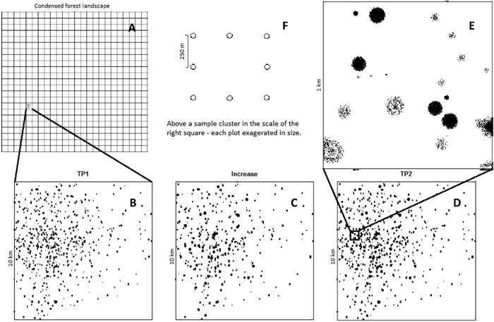
Fig. 1. Example of a simulated population in Scenario 2. The study area contains a total of 500 10×10 km squares. (A) A given proportion of these squares were chosen to contain damaged trees; the rest contained no damaged trees. Subfigures B-D show a single such 10×10 km square, with damaged trees indicated by black spots. Subfigure B shows a square containing 238 tree damage aggregation centres at the initial time point (TP1). Subfigure C shows an increment in which the intensity of all of the aggregation centres is increased, and 38 of them have increased in radius. Subfigure D shows the resulting population of damaged trees at a subsequent time point (TP2).
| Table 1. Parameters for the simulations of damaged trees in Scenario 1, with values set for simulated alternatives of damage level at an initial time point, TP1, and increases to a subsequent time point, TP2. | ||||
| TP1 | Sparse | Medium | ||
| Min no. trees ha–1 | 0.5 | 5 | ||
| Max no. trees ha–1 | 2.5 | 20 | ||
| Increase | Small | Large | Small | Large |
| Min new trees ha–1 | 0.05 | 9 | 0.5 | 38 |
| Max new trees ha–1 | 0.4 | 20 | 2 | 48 |
| Table 2. Parameters for simulations of damaged trees in Scenario 2, with values set for simulated alternatives of damage level at an initial time point, TP1, and increases to a subsequent time point, TP2. | ||||
| TP1 | Sparse | Medium | ||
| Min no aggregation centres square–1 | 200 | 500 | ||
| Max no aggregation centres square–1 | 800 | 1500 | ||
| Min aggregation centres radius (m) | 5 | 5 | ||
| Max aggregation centres radius (m) | 50 | 50 | ||
| Min no trees ha–1 within aggregation centres | 100 | 250 | ||
| Max no trees ha–1 within aggregation centres | 200 | 350 | ||
| Increase | Small | Large | Small | Large |
| Prob. change trees ha–1 in aggregation centres | 0.55 | 0.55 | 0.35 | 0.55 |
| Min change (relative to TP1) | 3 | 10 | 5 | 10 |
| Max change (relative to TP1) | 6 | 20 | 10 | 20 |
| Prob. change in aggregation centres radius | 0.15 | 0.15 | 0.05 | 0.15 |
| Min relative change in aggregation centres radius | 1.5 | 1.5 | 1.5 | 1.5 |
| Max relative change in aggregation centres radius | 2.0 | 2.0 | 2.0 | 2.0 |
| Table 3. Mean number of damaged trees ha–1, between square variance and mean within square variance for 100 simulated squares for each alternative of damage level in Scenario 1 and Scenario 2. | |||||
| Level at TP1 | Level of increase | Mean (trees ha–1) | Between square variance | Mean within square variance | |
| Scenario 1 | |||||
| TP1 | Sparse | Small | 1.5 | 0.4 | 6.1 |
| Large | 1.4 | 0.4 | 5.6 | ||
| Medium | Small | 11.6 | 17.0 | 44.3 | |
| Large | 12.7 | 15.8 | 48.3 | ||
| Increase | Sparse | Small | 0.2 | 0.0 | 0.8 |
| Large | 9.4 | 4.5 | 36.2 | ||
| Medium | Small | 1.2 | 0.2 | 4.8 | |
| Large | 35.6 | 31.4 | 130.2 | ||
| TP2 | Sparse | Small | 1.8 | 0.4 | 6.9 |
| Large | 10.8 | 5.2 | 41.5 | ||
| Medium | Small | 12.8 | 17.2 | 48.8 | |
| Large | 48.3 | 33.8 | 170.1 | ||
| Scenario 2 | |||||
| TP1 | Sparse | Small | 2.1 | 0.6 | 67.2 |
| Large | 2.0 | 0.6 | 63.2 | ||
| Medium | Small | 8.2 | 5.9 | 518.8 | |
| Large | 8.9 | 6.5 | 565.1 | ||
| Increase | Sparse | Small | 5.9 | 4.9 | 705.6 |
| Large | 17.0 | 42.2 | 7 046.6 | ||
| Medium | Small | 22.2 | 42.1 | 9 131.3 | |
| Large | 75.6 | 490.9 | 63 190.1 | ||
| TP2 | Sparse | Small | 8.0 | 9.0 | 1 073.0 |
| Large | 19.0 | 52.5 | 8 051.9 | ||
| Medium | Small | 30.4 | 79.0 | 12 241.5 | |
| Large | 84.4 | 609.2 | 72 560.0 | ||
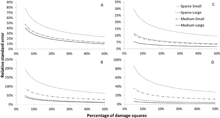
Fig. 2. Relative standard errors of estimators of the number of damaged trees ha–1 at a subsequent time point (TP2) (subfigs. A and C) and the increase, small and large increment, between the initial time point (TP1), at sparse and medium level, and TP2 (subfigs. B and D) for Scenario 1. Subfigures A and B show results obtained when using a sample consisting of a single year’s panel (n = 100), while subfigures C and D show results obtained using the full sample (N = 500).
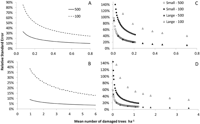
Fig. 3. Relative standard errors of estimators of the state at the initial time point (TP1; subfigs. A and B) and the increment, small and large, from TP1 to a subsequent time point (TP2; subfigs. C and D) in relation to the number of damaged trees ha–1 in Scenario 1 for the sparse (subfigs. A and C) and medium (subfigs. B and D) levels of tree damage at TP1. Results are shown for the full sample (N = 500) and a single year’s panel (n = 100).
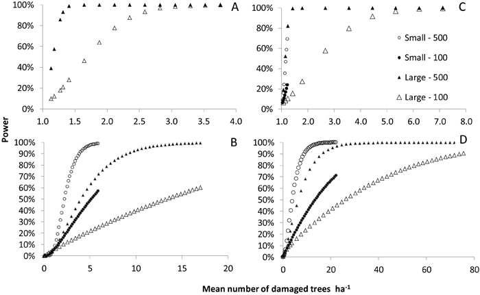
Fig. 4. The power to detect an increase in the number of damaged trees per hectare that exceeds 1 new damaged tree ha–1 in Scenario 1 (subfigs. A and C) and Scenario 2 (subfigs. B and D). Subfigs. A and B show the results for the sub-scenario with a sparse initial damage level while subfigs. B and D show the results for the sub-scenario with an intermediate initial damage level. Results are shown for a small and a large increment between the initial time point (TP1) and a subsequent time point (TP2). Data for the sub-scenario involving a small increment between TP1 and TP2 are omitted in the left hand figure, since the increase never exceeded 1 tree ha–1 in this case.