Silva Fennica

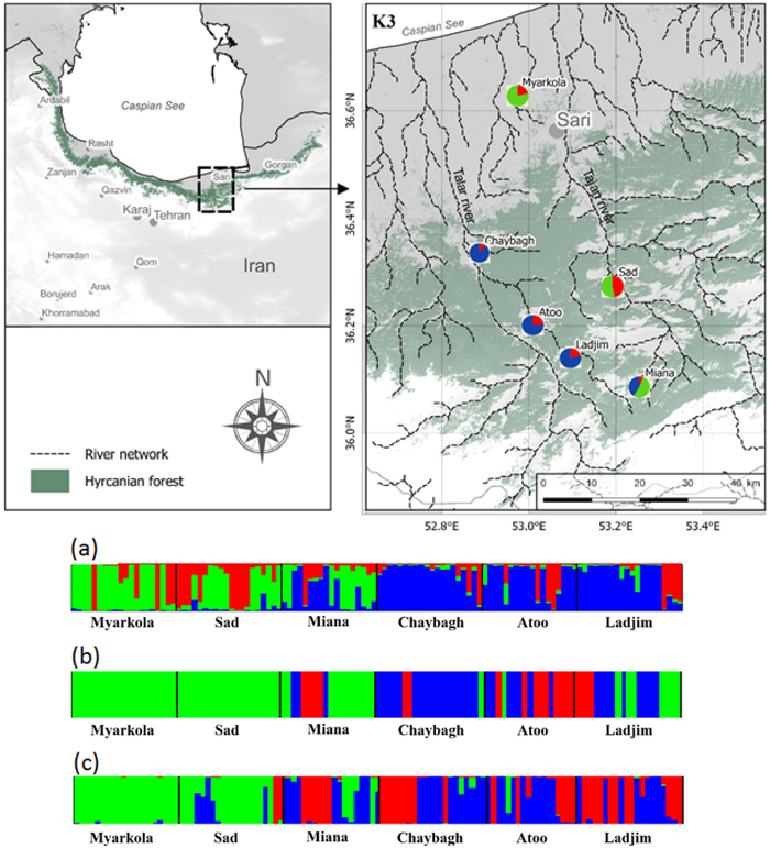
Fig. 1. Bayesian clustering results for Pterocarya fraxinifolia in the Hyrcanian region (N = 116) estimated along two altitudinal gradients from K = 3 and an associated map of the mean membership probabilities per site from STRUCTURE. Each individual is represented by a vertical bar partitioned into K segments, which represents the amount of ancestry of its genome corresponding to K clusters. Visualization was improved by sorting the genotypes by site. Gradient 1: Myarkola, Sad, and Miana; gradient 2: Chaybagh, Atoo, and Ladjim. (a) Output from STRUCTURE. (b) Output from BAPS. (c) Results of DAPC analysis in R.

Table 1. Geographical characteristics and sample size of investigated populations in two gradients along two river systems.
	Population name	Latitude (UTM)	Longitude (UTM)	Altitude (m a.s.l.)	Sample size
Tajan river (gradient 1)	Myarkola	672536.3	4051845.08	50–60	20
	Sad	697694.9	4017597.8	350–400	20
	Miana	703567.39	3996839.29	900–970	18
Talar river (gradient 2)	Chaybagh	669888.3	4023492.3	200–250	20
	Atoo	681346.47	4008915.14	400–450	18
	Ladjim	686691.74	4013147.26	900–950	20

Table 2. Genetic variability within two gradients of Pterocarya fraxinifolia populations.
	Elevation	Population	Effective number of alleles (Ne)	Observed heterozygosity (Ho)	Expected heterozygosity (He)	Allelic richness (Ar)	Private allelic richness (PAr)
Gradient 1	Low	Myarkola	5.7 ± 0.73	0.78 ± 0.1	0.807 ± 0.028	4.06	0.99
	Medium	Sad	4.7 ± 0.36	0.85 ± 0.067	0.78 ± 0.02	3.8	0.4
	High	Miana	5.1 ± 0.44	0.86 ± 0.07	0.79 ± 0.02	3.9	0.38
Gradient 2	Low	Chaybagh	3.72 ± 0.23	0.79 ± 0.11	0.726 ± 0.018	3.3	0.1
	Medium	Atoo	4.27 ± 0.51	0.87 ± 0.09	0.751 ± 0.025	3.5	0.2
	High	Ladjim	4.25 ± 0.69	0.86 ± 0.11	0.730 ± 0.043	3.4	0.14

Table 3. Analyses of molecular variance (AMOVA) for two gradients of Pterocarya fraxinifolia from Hyrcanian forest using SSR markers.
	AMOVA component						AMOVA genetic distance option
	S.O.V	d.f	SS	MS	Est. Var.	% of Variance	PhiPT	Rst	Fst	Nm
Gradient 1	Among Pops	2	27.76	13.8	0.45	9%	0.086**	0.049**	0.046**	5.13
	Within Pops	55	284.95	5.18	5.18	91%
	Total	57	312.72		5.63	100%
Gradient 2	Among Pops	2	22.13	11.06	0.34	7	0.075**	0.052**	0.036**	6.6
	Within Pops	55	237.68	4.32	4.32	93
	Total	57	259.82		4.67	100
Total	Among Pops	5	85.1	17	0.63	12	0.11**	0.037**	0.062**	3.77
	Within	110	521.3		4.7	88
	Total	115	606.4	4.7	5.37	100
Statistics include sums of squared deviations (SS); mean squared deviations (MS), variance component estimates (Est. Var.). ** – p-value < 0.01.

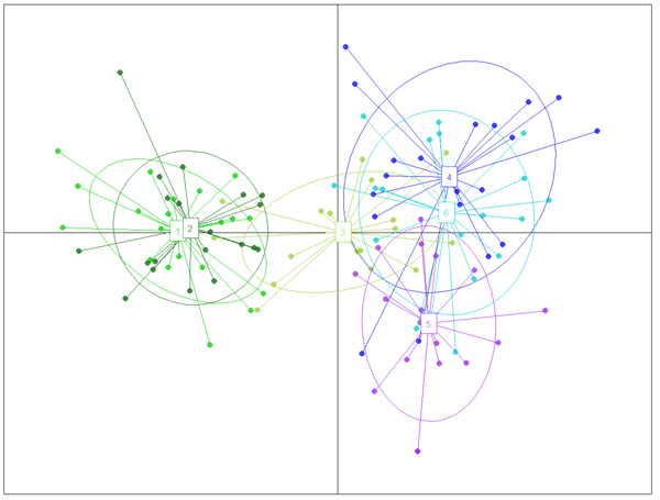
Fig. 2. The result of DAPC analysis with populations used as clusters: 1 – Myarkola, 2 – Sad, 3 – Miana, 4 – Chaybagh, 5 – Atoo, 6 – Ladjim. Green colours indicated populations from gradient 1, blue and purple – populations from gradient 2.

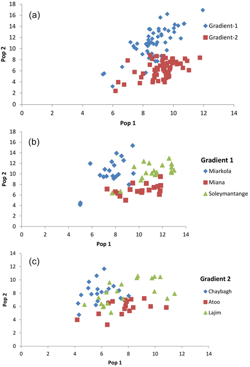
Fig. 3. Result of the population assignment. (a) Pairwise population assignment graphs of gradient 1 vs. gradient 2. (b) Assignment of the populations of gradient 1. (c) Assignment of the populations of gradient 2.

Table 4. Summary of population assignment outcomes to “self” or “other” population.
	Pop	Gradient 1 Pops	Gradient 2 Pops		Total	Percent
All populations*	Self Pop	52	57		109	94%
All populations*	Other Pop	6	1		7	6%
	Pop	Myarkola	Sad	Miana	Total	Percent
Gradient 1	Self Pop	17	20	18	55	95%
Gradient 1	Other Pop	3	0	0	3	5%
	Pop	Chaybagh	Atoo	Ladjim	Total	Percent
Gradient 2	Self Pop	18	16	16	50	86%
Gradient 2	Other Pop	2	2	4	8	14%
* – All population in each gradient grouped as one population.

Table 5. Pairwise population gene flow (Nm) values (below diagonal) and pairwise population genetic distance based on Fst values (above diagonal).
	Populations	Myarkola	Sad	Miana
Gradient 1	Myarkola	0.000	0.058	0.025
	Sad	9.88	0.000	4.343
	Miana	4.343	0.054	0.000
	Populations	Chaybagh	Atoo	Ladjim
Gradient 2	Chaybagh	0.000	0.041	0.026
	Atoo	5.856	0.000	0.043
	Ladjim	9.310	5.564	0.000
Nm – the product of the effective population number and rate of migration among populations.

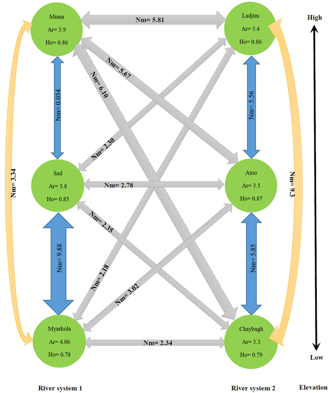
Fig. 4. Migration pattern of Pterocarya fraxinifolia within and among the river populations.