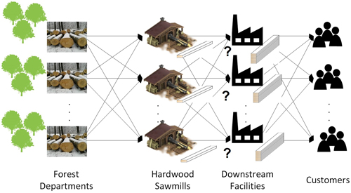
Fig. 1. The laminated beech wood supply network stakeholders and the material flows between them. There is a direct flow from one entity to all entities of the next tier. The source is at the forest departments and finishes at the sink, the customers. From several candidates, optimal downstream facilities are chosen to be opened within supply network.
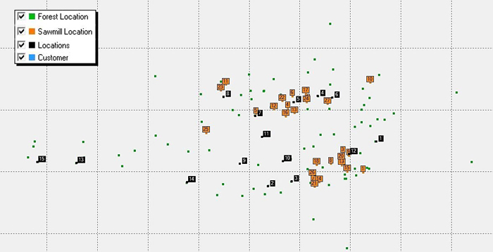
Fig. 2. The map represents the location of the several hardwood stakeholders. Forest departments with soft- and hardwood (green - 94), hardwood sawmills (orange - 27), laminated beech wood facility candidates (black -15) and customers (blue – have the same location as the forest departments - 88). View larger in new window/tab.
| Table 1. Countries and amounts for beech roundwood procurement. | |||||
| Country | City as central location | Share of beech in the country, estimated | Share of beech in the chosen location, estimated | Production, Sawlogs and veneer logs, non-coniferous* [m3 of roundwood] | Amount of beech in the chosen location, calculated [m3 of roundwood] |
| Slovakia | Nitra | 25% | 10% | 1 558 996 | 38 975 |
| Hungary | Székesfehérvár | 6% | 40% | 919 400 | 22 066 |
| Czech Republic | Iglau | 8% | 10% | 496 000 | 3968 |
| Germany | Landshut | 18% | 8% | 3 356 883 | 48 339 |
| Slovenia | Celje | 30% | 30% | 320 823 | 28 874 |
| Croatia | Zagreb | 36% | 10% | 1 958 567 | 70 508 |
| Total | 212 730 | ||||
| * FAOSTAT | |||||
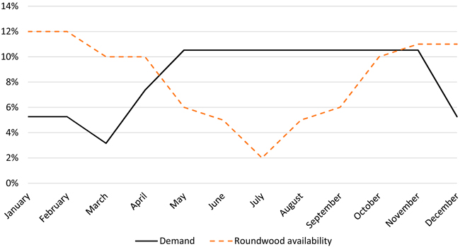
Fig. 3. Development of the annual product demand and the roundwood availability over the year.
| Table 2. Demand distribution key for Austria (Kaufmann et al. 2011), Italy and Germany. | ||||
| Countries | Scenario #1 – #13 | Scenario #14 | ||
| Federal States | Weighting [%] | Amount [m3] | Weighting [%] | Amount [m3] |
| Austria | 100.00 | 50 000 | 40.00 | 19 998 |
| Lower Austria | 21.52 | 10 760 | 21.52 | 4303 |
| Upper Austria | 17.01 | 8505 | 17.01 | 3403 |
| Styria | 16.53 | 8265 | 16.53 | 3306 |
| Vienna | 12.59 | 6295 | 12.59 | 2519 |
| Tyrol | 9.66 | 4830 | 9.66 | 1932 |
| Carinthia | 8.06 | 4030 | 8.06 | 1612 |
| Salzburg | 6.39 | 3195 | 6.39 | 1278 |
| Burgenland | 4.24 | 2120 | 4.24 | 844 |
| Vorarlberg | 4.00 | 2000 | 4.00 | 801 |
| Italy | 0 | 0 | 18.00 | 9000 |
| Germany | 0 | 0 | 42.00 | 21 000 |
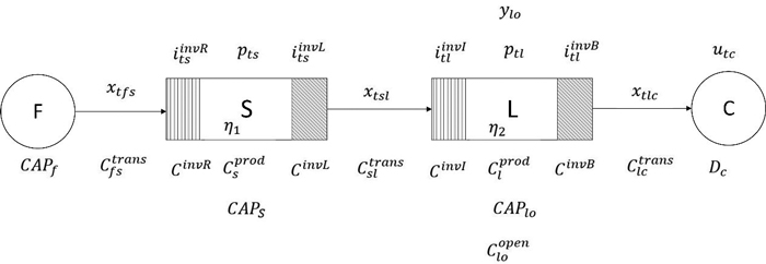
Fig. 4. Generic LBWSN with the four entities forest departments (F), hardwood sawmills (S), LBWF (L) and customers (C). I, p, u, x and y represent decision variables and the notations C and D represent parameters.
| Table 3. Developed scenarios with the defined parameters. | |||||
| Scenarios | Additional sawmill (ADS) | Amount of facilities (AF) | Facility capacity option (FCO) | Sourcing strategy (SO) | Amount of roundwood (AR) |
| #1 | unlimited | 3 | AUT | 146 023 | |
| #2 | unlimited | 3 | AUT | 146 023 | |
| #3 | unlimited | 3 | AUT | 146 023 | |
| #4 | unlimited | 6 | AUT | 146 023 | |
| #5 | x | unlimited | 3 | AUT | 146 023 |
| #6 | x | unlimited | 6 | AUT | 146 023 |
| #7 | x | unlimited | 3 | AUT + Neighbours | 358 762 |
| #8 | x | unlimited | 6 | AUT + Neighbours | 358 762 |
| #9 | x | 1 | 3 | AUT + Neighbours | 358 762 |
| #10 | x | 1 | 6 | AUT + Neighbours | 358 762 |
| #11 | unlimited | 3 | AUT + Neighbours | 358 762 | |
| #12 | x | unlimited | 3 | AUT + Neighbours | 358 762 |
| #13 | x | unlimited | 6 | AUT + Neighbours | 358 762 |
| #14 | x | unlimited | 6 | AUT + Neighbours | 358 762 |
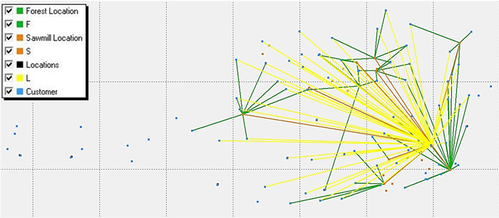
Fig. 5. Material flow of #1. The individual colours illustrate the material flows from forest locations to sawmills (green), from sawmills to facility locations (orange) and from facility location to customer (yellow).
| Table 4. Financial performance results for scenarios #1 to #14. | ||||||||||||||
| Cost parameter | #1 | #2 | #3 | #4 | #5 | #6 | #7 | #8 | #9 | #10 | #11 | #12 | #13 | #14 |
| Sadiesfied demand [m3] | 14 972 | 14 847 | 23 942 | 26 639 | 24 181 | 24 378 | 30 000 | 33 451 | 19 992 | 31 092 | 34 703 | 34 710 | 37 548 | 38 242 |
| Total supply cost per m3 [€ m–3] | 345 | 351 | 339 | 332 | 324 | 309 | 330 | 322 | 311 | 323 | 341 | 331 | 323 | 321 |
| Opening cost [€ m–3] | 48 | 49 | 53 | 41 | 53 | 30 | 49 | 33 | 46 | 30 | 47 | 47 | 34 | 27 € |
| Transport cost [€ m–3] | 109 | 121 | 79 | 86 | 71 | 76 | 87 | 94 | 70 | 92 | 92 | 87 | 92 | 93 € |
| Production cost [€ m–3] | 186 | 178 | 202 | 202 | 195 | 198 | 191 | 191 | 193 | 197 | 197 | 192 | 192 | 197 € |
| Storage cost [€ m–3] | 2 | 2 | 5 | 2 | 5 | 5 | 4 | 4 | 2 | 5 | 5 | 5 | 4 | 4 € |
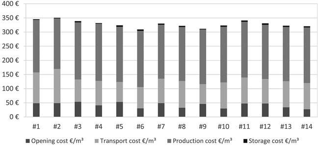
Fig. 6. The total supply network costs are represented per satisfied demand and for each sceanrio.
| Table 5. Material performance results for scenarios #1 to #14. | ||||||||||||||
| Material parameter | #1 | #2 | #3 | #4 | #5 | #6 | #7 | #8 | #9 | #10 | #11 | #12 | #13 | #14 |
| Degree of demand fulfillment [%] | 30 | 30 | 48 | 53 | 48 | 49 | 60 | 67 | 40 | 62 | 69 | 69 | 75 | 76 |
| Amount of used resources [%] | 49 | 49 | 78 | 87 | 79 | 80 | 40 | 45 | 27 | 41 | 46 | 46 | 50 | 51 |
| Amount of imported resources [%] | 0 | 0 | 0 | 0 | 0 | 0 | 25 | 27 | 6 | 17 | 25 | 24 | 27 | 28 |
| Amount of used sawmill capacity [%] | 54 | 61 | 42 | 46 | 37 | 37 | 45 | 51 | 30 | 23 | 27 | 26 | 28 | 28 |
| Amount of used LBWF capacity [%] | 100 | 99 | 60 | 78 | 69 | 98 | 100 | 98 | 100 | 91 | 99 | 87 | 88 | 75 |
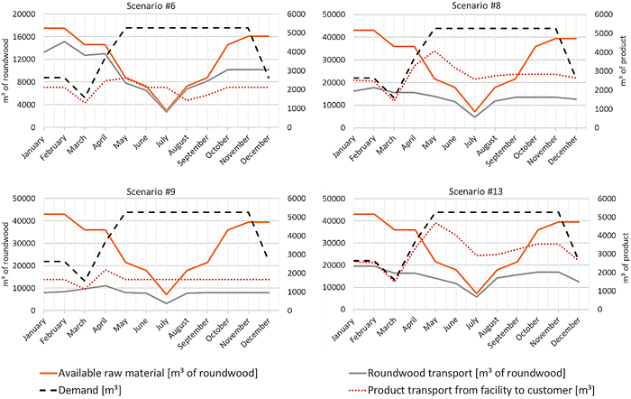
Fig. 7. Material performance results are shown for scenario 6, 8, 9 and 13. The raw material (orange,) and demand of products (black, m3 of product, right diagram title) curves result from the key distribution parameter and have the same development in the four diagrams. In contrast to the following three scenarios, #6 includes a national souring only. Roundwood (grey, m3 roundwood, left diagram title) product transportation (red, m3 of product, right diagram title) are the results of the individual scenarios. View larger in new window/tab.
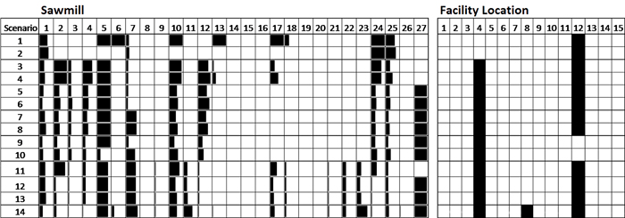
Fig. 8. For all 14 scenarios, the used sawmills and facilities are represented. For the facility locations, it is just shown if it is opened. The degree of sawmill capacity utilization is shown with percentage bar sizes. The additional sawmill 27 is used every time when it was possible.