| Table 1. Formulas for spatial explicit indices. | ||
| Index | Formulation | Explanations |
| CE (Clark and Evans 1954) | 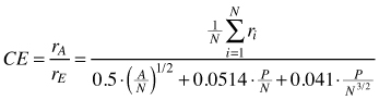 | rA – observed mean distances between trees A – area (m2) N – Total number of trees P – circumference of the plot |
| Tij (Kint 2004) | 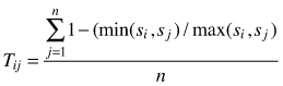 | si – size of i-th tree sj – size of j-th tree n – number of nearest neighbors (n = 3) |
| Uniform angle index Wi (Gadow and Hui 2002) |  | n – number of nearest neighbors vj = 1 if αj < α0 (α0 = 90°) otherwise: vj = 0 |
| Mean directional index Ri (Corral-Rivas et al. 2006) | 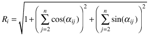 | αij – angle between i and j points |
| Index of nonrandomness Si (Pielou 1959) | λ – point density | |
| Mingling index SM (Gadow and Hui 2002) | 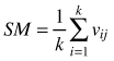 | k-numbers of nearest neighbors vij = 1 if reference tree and neighbor are different species, otherwise vij = 0 |
| Size dominance index Ui (Hui et al. 1998) |  | n – number of nearest neighbors vj = 0 if neighbor j is smaller than reference tree, otherwise vj = 1 |
| Dispersion index Iσ (Morisita 1962) | 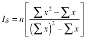 | n – sample size Σx – sum of quadrat counts (Σx)2 – sum of quadrat counts squared |
| Variance/mean ratio Ic (Krebs 1999) |  | Sn2 – variance |
| Mean of angles (Assunção 1994) |  | n – number of sampling points αi – angle between sample point and its nearest two neighbors |
| Segregation index (Pielou 1977) | m, n – numbers of species A and B | |
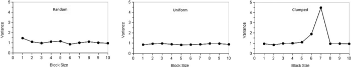
Fig. 1. Schematic illustration of the spatial pattern types for TTLQV method for contiguous quadrats: (left) random, (middle) regular and (right) clumped (adapted from Krebs 1999). View larger in new window/tab.
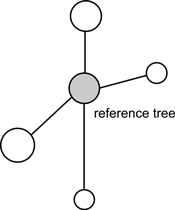
Fig. 2. An example of structural group of trees for calculation of uniform angle index (Wi), size differentiation index (T) and species mingling index (SM) (Pommerening 2002).
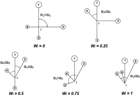
Fig. 3. Calculation of uniform angle index Wi and possible values for structural group of 4 neighbors around the reference i-tree (Gadow and Hui 2002).
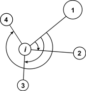
Fig. 4. Illustration of angle measurements for mean directional index Ri with structural group of 4 neighbors around the reference i-tree (Corral-Rivas et al. 2006).
| Table 2. Contingency table summarizing the number of trees of both species (A and B) with the nearest neighbors of their own species (a and d) and of the other species, used for Pielou’s segregation index calculation (Pielou 1977). | ||||
| Species of the nearest neighbor | ||||
| A | B | Total | ||
| Reference species | A | a | b | m |
| B | c | d | n | |
| Total | v | w | N | |
| Explanation: m = a + b; n = c + d; v = a + c; w = b + d; N = m + n | ||||
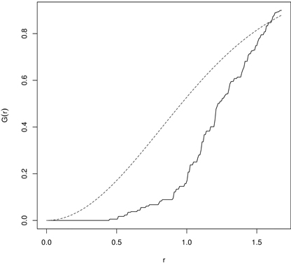
Fig. 5. The G-function calculated for 43 year old Scots pine semi-plantation indicating regularity (dashed line – the G-function for randomness (CSR); solid line – empirical G-function).
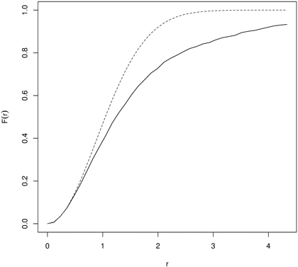
Fig. 6. The F-function for naturally regenerated English yew (Taxus baccata L.) trees indicating clustering (dashed line – the F-function for CSR; solid line – empirical F-function).
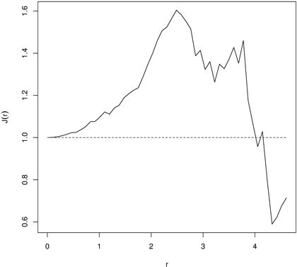
Fig. 7. The J-function indicating regular point pattern for 60 years old managed European beech stand indicating regularity (dashed line – the J-function for CSR; solid line – empirical J-function).
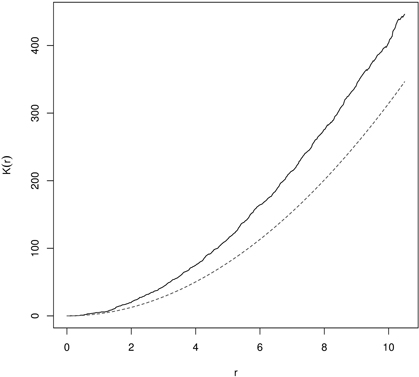
Fig. 8. Ripley’s K-function for English yew (males) trees indicating clumping distibution (dashed line – K-function for CSR; solid line – empirical K-function).
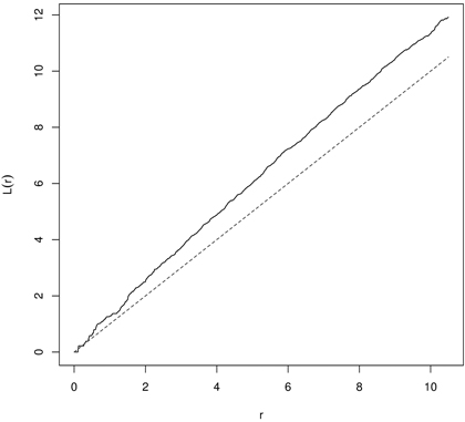
Fig. 9. The L-function for English yews (males) indicating clustering (dashed line – the L-function for CSR; solid line – empirical L-function).
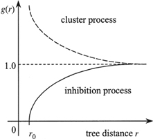
Fig. 10. Shape of pair correlation g-function for different types of point patterns (dashed line – the g-function for CSR; dashed line – clustering; solid line – regularity) (Pommerening 2002).
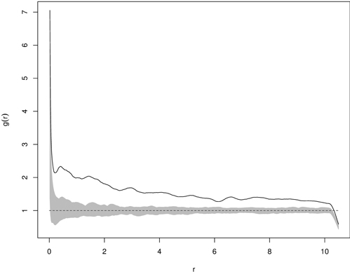
Fig. 11. Example of g(r) function for statistically significant clumped distribution of yew seedlings (solid line – empirical g-function; shaded area – critical region based on 199 Monte Carlo simulations; dashed line – g-function for CSR).
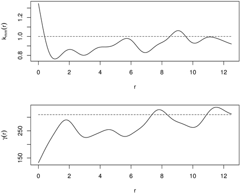
Fig. 12. Mark correlation function (kmm(r)) and mark variogram (γ(d)) for old-growth mixed forest (dashed line – independence in mark correlation; solid line – empirical functions).