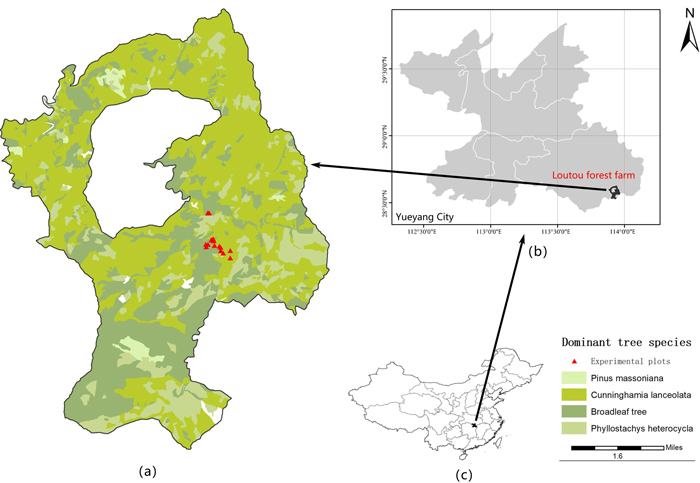
Fig. 1. The location of a) the study area – Loutou forest farm in b) Yueyang of Hunan Province, c) southern China. View larger in new window/tab.
| Table 1. The information of the measured variables for the 16 sample plots (Note: DBH: diameter at breat height; H: tree height; Cg: Cyclobalanopsis glauca; Rs: Rhododendron simsii; Cs: Castanopsis sclerophylla; Ce: Castanopsis eyriei; Lc: Loropetalum chinense; Cl: Cunninghamia lanceolate; Af: Alniphyllum fortune; Ca: Canarium album; Mr: Myrica rubra; Ss: Symplocos sumuntia). | |||||||||
| Sample plot number | Altitude (m) | Slope (degree) | Slope aspect | Slope position | Crown density | Tree composition | Number of trees | Mean DBH (cm) | Mean H (m) |
| 1 | 324 | 19 | sunny | medium | 0.9 | 4Cg 3Rs 1Cs 1Ce 1Lc | 63 | 15.4 | 11.1 |
| 2 | 340 | 17 | sunny | medium | 0.7 | 4Cg 3Rs 2Lc 1Cl | 54 | 12.9 | 9.5 |
| 3 | 312 | 22 | sunny | below | 0.8 | 4Cg 3Rs 2Cl 1Ce | 41 | 14.6 | 10.0 |
| 4 | 310 | 34 | shady | medium | 0.8 | 4Cg 4Rs 1Lc 1Ca | 54 | 12.5 | 9.3 |
| 5 | 330 | 20 | sunny | below | 0.7 | 3Cg 2Ce 2Cl 2Rs 1Mr | 30 | 14.9 | 9.7 |
| 6 | 312 | 32 | sunny | below | 0.8 | 4Cg 3Rs 2Ce 1Lc | 51 | 12.1 | 9.1 |
| 7 | 315 | 33 | sunny | below | 0.7 | 3Cg 3Af 3Rs 1Cl | 53 | 13.1 | 9.0 |
| 8 | 320 | 35 | shady | medium | 0.8 | 4Cg 3Cs 3Lc | 46 | 15.1 | 8.8 |
| 9 | 314 | 35 | shady | medium | 0.7 | 4Cg 2Cs 2Rs 1Af 1Lc | 29 | 14.3 | 11.3 |
| 10 | 318 | 32 | shady | upper | 0.7 | 5Cg 3Rs 2Af | 45 | 13.2 | 9.9 |
| 11 | 302 | 15 | shady | medium | 0.7 | 4Cg 2Af 2Cl 2Lc | 48 | 12.8 | 9.6 |
| 12 | 305 | 20 | shady | medium | 0.7 | 5Cg 2Rs 2Af 1Cl | 81 | 12.7 | 9.5 |
| 13 | 310 | 16 | shady | upper | 0.6 | 5Cg 2Rs 2Cs 1Lc | 50 | 12.3 | 12.5 |
| 14 | 325 | 27 | sunny | medium | 0.8 | 6Cg 2Cs 1Rs 1Cl | 52 | 14.6 | 9.5 |
| 15 | 308 | 30 | sunny | medium | 0.6 | 3Cg 3Cs 2Rs 1Ce 1Af | 40 | 9.5 | 9.6 |
| 16 | 285 | 20 | shady | below | 0.8 | 4Cg 3Cl 1Ce 1Af 1Rs | 100 | 12.1 | 10.3 |
| Table 2. Characteristics of Cyclobalanopsis glauca tree height and diameter at breast height (DBH) measurements for the total, modeling and validation datasets based on sunny-gentle, sunny-steep, shady-gentle and shady-steep (Max: maximum; Min: minimum; SD: standard deviation). | ||||||||||
| Subsets | Sample type | Number | Height (m) | DBH (cm) | ||||||
| Mean | Max | Min | SD | Mean | Max | Min | SD | |||
| Sunny-gentle | Total | 96 | 11.5 | 17.3 | 5.6 | 2.9 | 14.6 | 42.5 | 5.2 | 6.9 |
| Modeling | 77 | 11.5 | 17.3 | 5.6 | 3.0 | 14.7 | 42.5 | 5.2 | 7.3 | |
| Validation | 19 | 11.6 | 16.3 | 6.1 | 2.8 | 14.3 | 22.7 | 7.3 | 5.1 | |
| Sunny-s teep | Total | 86 | 10.3 | 15.4 | 6.5 | 2.2 | 12.9 | 26.0 | 5.0 | 5.1 |
| Modeling | 69 | 10.2 | 15.4 | 6.5 | 2.3 | 13.0 | 26.0 | 5.0 | 5.4 | |
| Validation | 17 | 10.5 | 14.4 | 7.8 | 1.8 | 12.4 | 18.6 | 6.1 | 4.1 | |
| Shady-gentle | Total | 139 | 10.4 | 14.9 | 3.5 | 2.5 | 12.8 | 29.0 | 5.1 | 4.9 |
| Modeling | 111 | 10.4 | 14.8 | 3.5 | 2.5 | 12.9 | 27.2 | 5.1 | 4.9 | |
| Validation | 28 | 10.4 | 14.9 | 5.8 | 2.5 | 12.0 | 29.0 | 5.8 | 4.7 | |
| Shady- steep | Total | 105 | 10.6 | 15.0 | 6.4 | 2.0 | 15.2 | 41.6 | 5.1 | 7.0 |
| Modeling | 84 | 10.7 | 14.7 | 6.4 | 1.9 | 14.8 | 33.4 | 5.1 | 6.3 | |
| Validation | 21 | 10.2 | 15.0 | 6.7 | 2.4 | 16.4 | 41.6 | 5.1 | 9.4 | |
| Table 3. The basic models used for comparison of modeling the relationship of tree height (H) with diameter at breast height (DBH) (Note: D is DBH; a, b, c and d are model parameters; M#: model numbers). | |||||
| M# | Model | References | M# | Model | References |
| M1 | Linear | M7 | Yoshida (1928) | ||
| M2 | Log | M8 | Schumacher (1939) | ||
| M3 | Exponential | M9 | Richards (1959) | ||
| M4 | Hyperbolic curve | M10 | Huang and Titus (1992) | ||
| M5 | Quadratic | M11 | Wykoff et al. (1982) | ||
| M6 | Gompertz (1825) | ||||
| Table 4. The results of eleven basic models (M1 to M11) used for fitting the H-DBH relationship using the whole modeling dataset (H is tree height; DBH is diameter at breast height; a, b, c and d are model parameters; RMSE and R2 respectively are root mean square error and coefficient of determination between the observed and estimated values of H; and SSR is the sum of squared residuals). | |||||||
| Model parameter | Model evaluation | ||||||
| M# | a | b | c | d | R2 | SSR | RMSE |
| M1 | 0.321 | 6.241 | 0.624 | 972.654 | 1.511 | ||
| M2 | 4.735 | –1.323 | 0.683 | 821.522 | 1.389 | ||
| M3 | 3.529 | 0.043 | 0.670 | 854.983 | 1.417 | ||
| M4 | 19.897 | 216.848 | 10.988 | 0.685 | 816.203 | 1.384 | |
| M5 | –0.0097 | 0.6517 | 3.8716 | 0.679 | 831.126 | 1.397 | |
| M6 | 15.02 | 1.471 | 0.116 | 0.686 | 813.143 | 1.382 | |
| M7 | 10.672 | 156.574 | 2.024 | 5.169 | 0.686 | 811.589 | 1.380 |
| M8 | 16.936 | 5.552 | 0.676 | 839.931 | 1.404 | ||
| M9 | 15.949 | 0.764 | 0.071 | 0.685 | 814.723 | 1.383 | |
| M10 | 0.874 | 0.235 | 0.682 | 821.891 | 1.389 | ||
| M11 | 2.87 | –6.62 | 0.681 | 826.471 | 1.393 | ||
| Table 5. The results of the optimal models selected from the eleven basic models (M1 to M11) used for fitting the H-DBH relationship for each of the sub-datasets including sunny, shady, steep and gentle slope, and sunny-steep, sunny-gentle, shady-steep and shady-steep (a, b and c are model parameters; RMSE and R2 respectively are root mean square error and coefficient of determination between the observed and estimated values of H; SSR is the sum of squared residuals; and AIC is Akaike information criterion). | ||||||||
| Dataset | Model # | Model parameter | Model evaluation | |||||
| a | b | c | R2 | SSR | RMSE | AIC | ||
| Sunny slope | M6 | 16.704 | 1.416 | 0.094 | 0.695 | 394.29 | 1.472 | 146.7 |
| Shady slope | M6 | 13.945 | 1.597 | 0.140 | 0.702 | 379.41 | 1.247 | 113.7 |
| Steep slope | M2 | 3.922 | 0.451 | 0.714 | 232.83 | 1.104 | 85.4 | |
| Gentle slope | M6 | 15.816 | 1.757 | 0.124 | 0.720 | 492.06 | 1.447 | 130.3 |
| Sunny-steep | M2 | 4.253 | –0.249 | 0.622 | 154.55 | 1.341 | 54.4 | |
| Sunny-gentle | M6 | 16.817 | 1.591 | 0.109 | 0.754 | 200.08 | 1.444 | 76.5 |
| Shady-steep | M3 | 4.094 | 0.359 | 0.818 | 73.03 | 0.834 | –34.1 | |
| Shady-gentle | M6 | 14.119 | 2.184 | 0.169 | 0.706 | 255.58 | 1.356 | 92.7 |
| Table 6. The comparison of the results using the optimal models without and with the original Hegyi and improved Hegyi_I involved for sunny-steep, sunny-gentle, shady-steep and shady-gentle slope forests (a, b, c, f and g are model parameters; STE is the standard error of the estimated parameter; RMSE and R2 respectively are root mean square error and coefficient of determination between the observed and estimated values of H; SSR is the sum of squared residuals; and the symbol * implying the model parameter statistically is significantly different from zero at the significant level of 0.05). | ||||||||
| Model characteristics | Model parameter | Model evaluation | ||||||
| a (STE) | b (STE) | c (STE) | f (STE) | g (STE) | RMSE | SSR | R2 | |
| Sunny-steep slope | ||||||||
| *4.253(0.362) | –0.249(0.908) | 1.341 | 154.550 | 0.622 | ||||
| *10.198(0.906) | –0.921(1.083) | 0.071(0.063) | 1.330 | 152.192 | 0.628 | |||
| *3.693(0.463) | 1.712(1.367) | *–0.182(0.086) | 1.312 | 148.219 | 0.638 | |||
| Sunny-gentle slope | ||||||||
| *16.817(0.924) | *1.591(0.178) | *0.109(0.019) | 1.444 | 200.078 | 0.754 | |||
| *16.858(0.981) | *1.542(0.283) | *0.107(0.022) | 0.006(0.026) | 1.443 | 199.967 | 0.754 | ||
| *17.259(0.967) | *1.119(0.130) | *0.093(0.016) | *0.015(0.004) | 1.348 | 174.524 | 0.786 | ||
| Shady-steep slope | ||||||||
| *4.094(0.195) | *0.359(0.017) | 0.834 | 73.031 | 0.818 | ||||
| *4.415(0.245) | *0.339(0.018) | *–0.022(0.009) | 0.811 | 69.059 | 0.828 | |||
| *4.864(0.279) | *0.316(0.018) | *–0.017(0.004) | 0.759 | 60.472 | 0.849 | |||
| Shady-gentle slope | ||||||||
| *14.119(0.581) | *2.184(0.355) | *0.169(0.026) | 1.356 | 255.579 | 0.706 | |||
| *14.301(0.645) | *1.928(0.402) | *0.162(0.029) | –0.298(0.250) | 1.363 | 258.098 | 0.703 | ||
| *13.906(0.504) | *2.850(0.569) | *0.191(0.027) | *–0.044(0.021) | 1.341 | 249.868 | 0.712 | ||
| Table 7. Significant difference test of the average absolute residuals from zero using the models without and with the competition indices Hegyi CI and Hegyi_I CI involved (δ1 is the average of the absolute residuals for the model without competition index, δ2 is the average of the absolute residuals for the model with the original Hegyi and δ3 is the average of the absolute residuals for the model with the improved Hegyi_I). | ||||||||||
| Sub-datasets | Model | δ1 | δ2 | δ3 | δ1 vs. δ2 | δ1 vs. δ3 | δ2 vs. δ3 | |||
| T value | P value | T value | P value | T value | P value | |||||
| Sunny-steep | M2 | 1.10* | 1.05* | 0.98* | 1.635 | 0.106 | 2.310 | 0.023 | 1.578 | 0.118 |
| Sunny-gentle | M6 | 1.18* | 1.12* | 1.09* | 0.405 | 0.686 | 1.748 | 0.084 | 0.303 | 0.763 |
| Shady-steep | M3 | 0.65* | 0.62* | 0.57* | 1.292 | 0.199 | 2.386 | 0.019 | 1.903 | 0.060 |
| Shady-gentle | M6 | 1.11* | 1.09* | 1.05* | 0.676 | 0.500 | 1.906 | 0.059 | 1.495 | 0.137 |
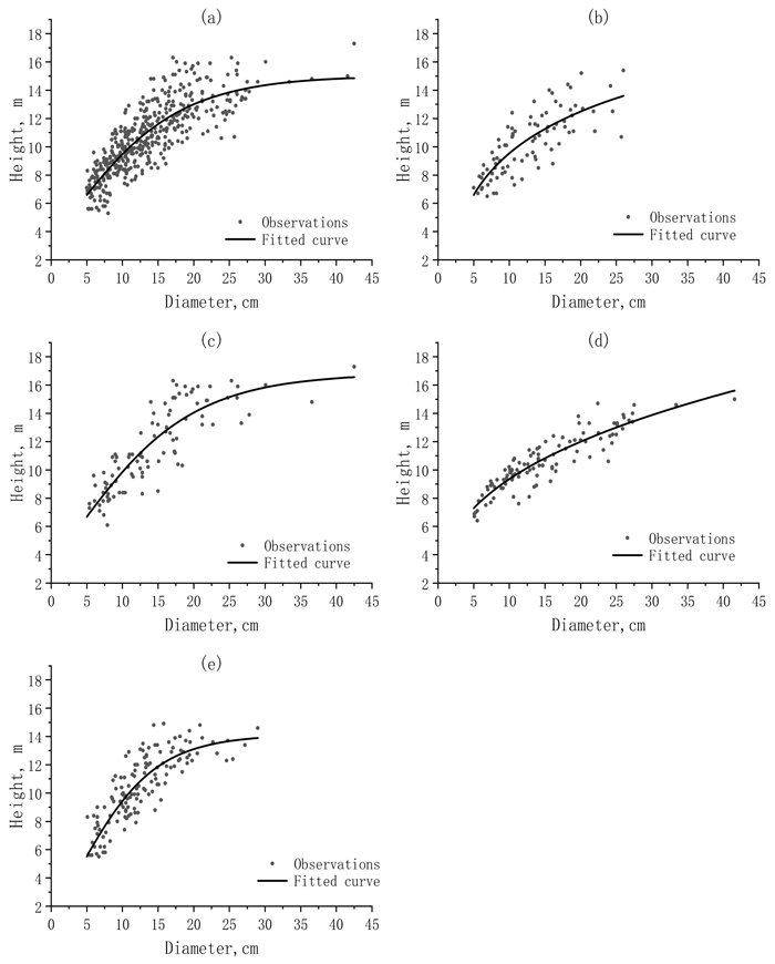
Fig. 2. The scattered distributions and fitted curves of the observed height (H) against the observed diameter (DBH) for a) the whole dataset and different sub-datasets: b) sunny-steep; c) sunny-gentle; d) shady-steep; and e) shady-gentle.
| Table 8. The improvement of tree H predictions using separate models at different slopes and aspects by comparison with the whole model based on root mean square error (RMSE) between the predicted and observed values of the validation dataset (W is the whole model, S1 is the separate models without competition index, S2 is the separate models with the original Hegyi and S3 is the separate models with the improved Hegyi_I. | ||||||||
| Datasets | RMSE | Percentage of reduced error (%) | ||||||
| W | S1 | S2 | S3 | W vs. S1 | W vs. S2 | W vs. S3 | S2 vs. S3 | |
| Sunny-steep slope | 1.366 | 1.341 | 1.33 | 1.312 | 1.83 | 2.64 | 3.95 | 1.35 |
| Sunny-gentle slope | 1.635 | 1.444 | 1.443 | 1.348 | 11.68 | 11.74 | 17.55 | 6.58 |
| Shady-steep slope | 1.064 | 0.834 | 0.811 | 0.759 | 21.62 | 23.78 | 28.66 | 6.41 |
| Shady-gentle slope | 1.412 | 1.356 | 1.363 | 1.341 | 3.97 | 3.47 | 5.03 | 1.61 |