| Table 1. The fixed-effects ingrowth model for Scots pine estimated with the zeroinfl function in R package pscl. The function estimates the dispersion parameter in form log(1/α). G is the stand basal area, VT and CT are the indicator variables for sub-xeric and xeric or poorer forest types. Log(T) and log(A) are used as offsets, where A = 100 m2 is the area of plot and T = 5 yrs is the length of the growth period. |
| Predictor | Estimate | Std. Error | Pr(>|z|) |
| Count model (negative binomial with log link) |
| log(T) | 1 | | |
| log(A) | 1 | | |
| Intercept | –6.82 | 0.41 | <2e–16 |
| Gpine | –0.131 | 0.112 | 0.023 |
 | 0.783 | 0.308 | 0.011 |
| VT | 0.633 | 0.250 | 0.011 |
| CT | 1.64 | 0.34 | 1.2e–06 |
| ln(1/α) | –1.16 | 0.209 | |
| Zero-inflation model coefficients (binomial with logit link) |
| Intercept | –13.6 | 3.5 | 0.0001 |
| ln(Gpine + 0.01) | –0.307 | 0.083 | 0.00021 |
| √G | 6.1 | 1.5 | 5.9E–05 |
| G | –0.58 | 0.16 | 0.0003 |
| VT | –1.21 | 0.36 | 0.00075 |
| Table 2. The fixed-effects ingrowth model for Norway spruce. OMT is an indicator variable for herb-rich or better site. TS is the temperature sum. The other symbols are as in Table 1. |
| Predictor | Estimate | Std. Error | Pr(>|z|) |
| Count model (negative binomial with log link) |
| log(T) | 1 | | |
| log(A) | 1 | | |
| Intercept | –6.61 | 0.54 | <2e–16 |
| log(Gspruce + 0.01) | 0.148 | 0.029 | 2.9e–07 |
| max(Gspruce – 13.0) | –0.0207 | 0.0109 | 0.056 |
| TS | 0.00126 | 0.00048 | 0.0082 |
| log(1/α) | –0.83 | 0.11 | |
| Zero-inflation model coefficients (binomial with logit link) |
| Intercept | –1.75 | 0.46 | 8.6e–05 |
| log(Gspruce + 0.01) | –0.359 | 0.073 | 9.0e–07 |
| OMT | 1.12 | 0.43 | 0.0085 |
| CT | 1.10 | 0.48 | 0.021 |
| Table 3. The fixed-effects ingrowth model for birch (combined ingrowth of silver and downy birch). The symbols are as in Table 1. |
| Predictor | Estimate | Std. Error | Pr(>|z|) |
| Count model (negative binomial with log link) |
| log(T) | 1 | | |
| log(A) | 1 | | |
| Intercept | –3.15 | 0.18 | <2e–16 |
| Gpine | 0.0923 | 0.0090 | <2e–16 |
| Gbirch | –0.109 | 0.045 | 0.016 |
| √Gbirch | 0.349 | 0.150 | 0.020 |
| G | –0.113 | 0.0091 | <2e–16 |
| VT | –0.50 | 0.16 | 0.0016 |
| CT | –0.87 | 0.29 | 0.0032 |
| log(1/α) | –1.013 | 0.092 | |
| Zero-inflation model (binomial with logit link) |
| Intercept | –6.40 | 1.57 | 0.000044 |
| log(Gbirch + 0.01) | –0.565 | 0.17 | 0.00078 |
| G | 0.142 | 0.033 | 0.000014 |
| VT | 0.822 | 0.51 | 0.11 |
| CT | 2.41 | 0.75 | 0.0014 |
| Table 4. Statistics for the fixed-effects ingrowth models. Row “P(Residual > 0)” gives the proportion of positive residuals. |
| Variable | Minimum | Maximum | Mean | sd |
| Scots pine |
| Ingrowth | 0 | 68 | 0.90 | 4.07 |
| Censored ingrowth | 0 | 5 | 0.457 | 1.26 |
| Probability of extra zeroes (p) | 0.0009 | 0.97 | 0.68 | 0.28 |
| Prediction | 0.018 | 8.10 | 0.890 | 1.38 |
| Residual | –8.10 | 64.34 | –0.0016 | 3.89 |
| P(Residual > 0) | | | 0.11 | |
| Pearson residual | –0.55 | 28.79 | –0.0020 | 1.13 |
| Censored prediction | 0.017 | 2.39 | 0.47 | 0.52 |
| Censored residual | –2.37 | 4.90 | –0.001 | 1.15 |
| Censored Pearson residual | –1.05 | 9.91 | –0.007 | 0.93 |
| Norway spruce |
| Ingrowth | 0 | 47 | 2.61 | 5.3 |
| Censored ingrowth | 0 | 5 | 1.47 | 1.95 |
| Probability of extra zeroes (p) | 0.04 | 0.74 | 0.22 | 0.20 |
| Prediction | 0.27 | 5.0 | 2.60 | 1.29 |
| Residual | –4.84 | 43.6 | 0.010 | 5.16 |
| P(Residual > 0) | | | 0.27 | |
| Pearson residual | –0.61 | 12.97 | 0.0010 | 1.08 |
| Censored prediction | 0.24 | 2.27 | 1.49 | 0.59 |
| Censored residual | –2.25 | 4.71 | –0.022 | 1.84 |
| Censored Pearson residual | –1.04 | 4.97 | –0.014 | 0.98 |
| Birch (silver birch and downy birch) |
| Ingrowth | 0 | 120 | 5.45 | 12.8 |
| Censored ingrowth | 0 | 5 | 1.77 | 2.14 |
| Probability of extra zeroes (p) | 0.0015 | 0.940 | 0.17 | 0.21 |
| Prediction | 0.035 | 23.4 | 5.33 | 4.29 |
| Residual | –19.4 | 102.7 | 0.12 | 11.7 |
| P(Residual > 0) | | | 0.25 | |
| Pearson residual | –0.60 | 11.4 | –0.0023 | 1.02 |
| Censored prediction | 0.035 | 3.31 | 1.75 | 0.80 |
| Censored residual | –3.19 | 4.48 | 0.023 | 1.95 |
| Censored Pearson residual | –1.47 | 6.03 | 0.0098 | 1.00 |
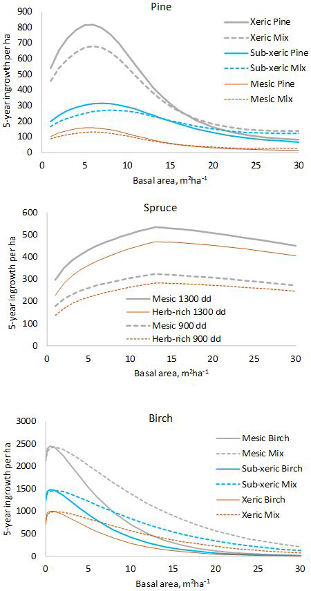
Fig. 1. Five-year predictions calculated with the fixed-effects model shown in Tables 1–3. log(10000) and log(5) were used as offsets to obtain per-hectare values for five years. In the diagram for pine, “Mix” refers to a stand where 50% of the basal area is pine and 50% is other species. In the diagram for birch, “Mix” is a stand where 50% of the basal area is birch and 50% is pine.
| Table 5. The mixed-effects ingrowth model for Scots pine. VT is the sub-xeric type, and CT is the xeric type. |
| Predictor | Estimate | Std. Error | Pr(>|z|) |
| Conditional model |
| log(T) | 1 | | |
| log(A) | 1 | | |
| Intercept | –6.47 | 0.56 | <2e–16 |
| ln(Gpine + 0.01) | 0.323 | 0.074 | 1.4E–05 |
| √G | –1.04 | 0.13 | 6.4E–15 |
| VT | 0.73 | 0.23 | 0.0018 |
| CT | 1.23 | 0.37 | 0.00082 |
| Zero-inflation model |
| Intercept | –5.40 | 0.88 | 8.6e–10 |
| Table 6. The mixed-effects ingrowth model for Norway spruce. TS is the temperature sum and CT is the xeric type. |
| Predictor | Estimate | Std. Error | Pr(>|z|) |
| Count model |
| log(T) | 1 | | |
| log(A) | 1 | | |
| Intercept | –7.58 | 0.69 | <2e–16 |
| ln(Gspruce + 0.01) | 0.287 | 0.032 | <2e–16 |
| max(Gspruce – 13.0) | –0.0532 | 0.0126 | 2.4e–05 |
| LS | 0.000716 | 0.00060 | 0.235 |
| Zero-inflation model |
| Intercept | –3.74 | 0.27 | <2e–16 |
| ln(Gspruce + 0.01) | –0.32 | 0.12 | 0.0096 |
| CT | 1.31 | 1.02 | 0.20 |
| Table 7. The mixed-effects ingrowth model for birch. |
| Predictor | Estimate | Std. Error | Pr(>|z|) |
| Conditional model |
| log(T) | 1 | | |
| log(A) | 1 | | |
| Intercept | –4.27 | 0.20 | <2e–16 |
| G | –0.127 | 0.010 | <2e–16 |
| log(Gbirch + 0.01) | 0.221 | 0.030 | 1.6e–13 |
| Gpine | 0.0815 | 0.0107 | 2.7e–14 |
| CT | –0.21 | 0.19 | 0.26 |
| Zero-inflation model |
| Intercept | –5.03 | 0.86 | 4.2e–09 |
| G | 0.0929 | 0.033 | 0.004 |
| Table 8. Statistics for the mixed-effects ingrowth models. Notations (11) and (12) refer to Eqs. 11 and 12, respectively. |
| Variable | min | max | mean | sd |
| Scots pine |
| Probability of extra zeroes (p) | 0.0045 | 0.0045 | 0.0045 | 0 |
| Prediction | 0.0001 | 0.767 | 0.039 | 0.072 |
| Prediction | 0.010 | 82.91 | 4.21 | 7.84 |
| Residual (11) | –0.6668 | 67.87 | 0.8567 | 4.05 |
| P(Residual (11) > 0) | | | 0.16 | |
| Residual (12) | –72.12 | 54.48 | –3.318 | 7.60 |
| P(Residual(12) > 0) | | | 0.055 | |
| Pearson residual (11) | –8.01E–05 | 0.260 | 0.002 | 0.012 |
| Pearson residual (12) | –0.0087 | 0.252 | –0.007 | 0.012 |
| Censored prediction | 0.0075 | 1.86 | 0.390 | 0.335 |
| Censored residual | –1.80 | 4.83 | 0.068 | 1.17 |
| Censored Pearson residual | –0.84 | 6.80 | 0.019 | 0.94 |
| Norway spruce |
| Probability of extra zeroes (p) | 0.0068 | 0.277 | 0.042 | 0.060 |
| Prediction | 0.090 | 1.37 | 0.695 | 0.382 |
| Prediction | 0.45 | 6.83 | 3.47 | 1.90 |
| Residual (11) | –1.30 | 46.27 | 1.91 | 5.25 |
| P(Residual(11) > 0) | | | 0.43 | |
| Residual (12) | –6.47 | 43.37 | –0.86 | 5.20 |
| P(Residual(12) > 0) | | | 0.24 | |
| Pearson residual (11) | –0.040 | 6.560 | 0.12 | 0.39 |
| Pearson residual (12) | –0.20 | 6.41 | –0.038 | 0.39 |
| Censored prediction | 0.33 | 2.07 | 1.34 | 0.54 |
| Censored residual | –2.02 | 4.64 | 0.13 | 1.85 |
| Censored Pearson residual | –0.99 | 4.81 | 0.070 | 1.07 |
| Birch (silver birch and downy birch) |
| Probability of extra zeroes (p) | 0.0074 | 0.45 | 0.055 | 0.050 |
| Prediction (11) | 0.0070 | 5.50 | 1.18 | 1.09 |
| Prediction (12) | 0.058 | 45.5 | 9.79 | 9.00 |
| Residual (11) | –5.23 | 117.2 | 4.27 | 12.4 |
| P(Residual(11) > 0) | | | 0.43 | |
| Residual (12) | –43.3 | 96.7 | –4.35 | 12.9 |
| P(Residual(12) > 0) | | | 0.18 | |
| Pearson residual (11) | –0.014 | 2.30 | 0.057 | 0.17 |
| Pearson residual (12) | –0.12 | 2.20 | –0.041 | 0.17 |
| Censored prediction | 0.052 | 3.27 | 1.63 | 0.75 |
| Censored residual | –3.22 | 4.57 | 0.142 | 1.98 |
| Censored Pearson residual | –1.55 | 4.81 | 0.080 | 1.07 |
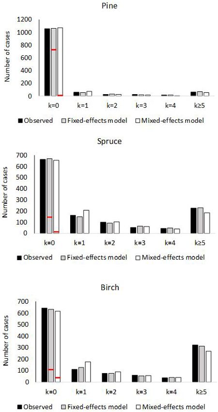
Fig. 2. Number of plots with 0, 1, 2, 3, 4 or ≥5 ingrowth trees based on observed and predictedingrowth. The marginal distribution of the predicted ingrowth is computed using Eq. 1. The frequency of extra zeros is shown with the red horizontal line.
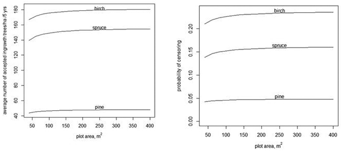
Fig. 3. The average number of accepted ingrowth trees per ha when the censoring limit is 500 trees per ha, i.e., the censored variable is min(y, ) (left) and the average probablity that some ingrowth trees within a plot are censored when 500 trees/ha are accepted (right).
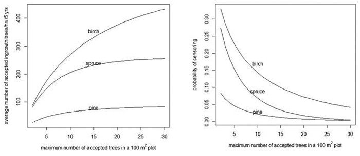
Fig. 4. Average number of acceptable ingrowth trees/ha in 5 years (left) and the probability that some trees are censored in a 100 m2 plot (right) as a function of the maximum number of acceptable trees in a 100 m2 plot. As a reference, note that without censoring there are 90, 259 and 524 trees/ha for pine, spruce and birch, respectively (see the "Prediction" rows of Table 4).