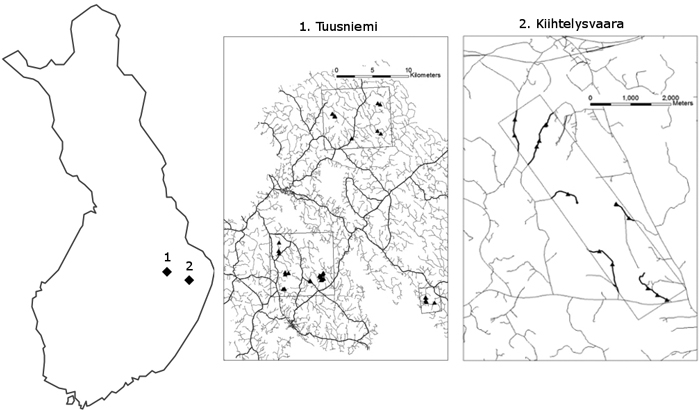
Fig. 1. The locations of the areas examined during the field inventories of unpaved forest road quality assessments. Both Tuusniemi and Kiihlelysvaara are located in the Finnish Lakeland region in Eastern Finland.
| Table 1. The road quality variables (structural condition, surface wearing and flatness) collected based on a Finnish Forest Road Quality recommendations (Korpilahti 2008) developed by Metsäteho Oy were classified to three quality categories in the study. The simplified table lists the road problems to be included in each category and the empirical assessment factors for good, satisfactory, and poor classes. | ||||
| Assessed roads quality variables | Road quality issues to pay attention while assessing each variable | Road quality classes | ||
| Good | Satisfactory | Poor | ||
| Structural condition | The whole road body condition. Visibility of driving lines. | The road surface is smooth; therefore, the driving speed does not need to be reduced | Some road quality problems (such as ruts) are visible, driving lines must be chosen with care and speeds have to be slightly reduced. | There are clearly visible ruts so the driving lines must be chosen carefully, and driving speeds have to be significantly reduced. |
| Surface wearing | The road wearing layer’s quality and material (fine, coarse, not present). | The road’s wearing layer is sufficiently thick and of good quality. | The wear layer is too thin, or the material is either too fine or too coarse. These are hindering vehicle movement and require slightly reduced speed. | The wear layer has majorly been worn away, or the material is too fine or too coarse. These factors are significantly hindering driving and speed reduction is necessary. |
| Flatness | The evenness of the road surface. Depressions, grooves and side bulges are present or not. Road drainage status. | The road has an even surface. There is no risk or damage to vehicles. The drainage of the surface is good. Road conditions will not hinder transportation or daily movement. | The wear layer is uneven, and the road has depressions, grooves and lateral bulges. There is visible damage. Lower speeds may be required in some places, but the risk of damage to a vehicle is quite small and will not hinder transportation or daily movement. | The road has depressions, grooves and lateral bulges, and/or drainage of its surface does not function well. The wear layer is defective, and driving conditions are obviously poor. It is necessary to reduce speed and to change the driving line frequently to avoid vehicle damage. The poor condition of the road hinders transportation and daily movement. |
| Table 2. Distribution of field observations between the road quality classes (poor, satisfactory and good) of road sections in two study areas. In Tuusniemi all 3 road quality classes were present, while in Kiihtelysvaara the road quality was better and only 2 classes were present. | ||||
| Tuusniemi, year 2014 | ||||
| Road quality class | Structural condition | Surface wearing | Flatness | Total number of road sections of each road quality class |
| Poor | 3 | 6 | 3 | 12 |
| Satisfactory | 13 | 27 | 22 | 62 |
| Good | 33 | 16 | 24 | 73 |
| Total number of road sections of each road quality parameter | 49 | 49 | 49 | 147 |
| Kiihtelysvaara, year 2013 | ||||
| Road quality class | Structural condition | Surface wearing | Flatness | Total number of road sections of each road quality class |
| Poor | 0 | 0 | 0 | 0 |
| Satisfactory | 3 | 7 | 6 | 16 |
| Good | 10 | 6 | 7 | 23 |
| Total number of road sections of each road quality parameter | 13 | 13 | 13 | 39 |
| Table 3. List of variables tested for prediction. In the table, dz: distance of height values from the reference DEM; dz5: distance of 5 random height values from the reference DEM SP: spline interpolation; KR: kriging interpolation; IDW: inverse distance-weighted interpolation; NN: natural neighbour interpolation. Topographic Position Indices (TPI) and Standardized Elevation (SE) names are the following: Interpolation Technique for Reference DEM ‘_’ Interpolation for Surface Quality Index. | ||
| ALS derived values – applied for height values in one cell | Reference DEM interpolation methods | Interpolation methods used for DEMs for TPI and SE calculations |
| intensity | SP | SP |
| range | KR | KR |
| variance | IDW | IDW |
| dz | NN | NN |
| dz^2 | ||
| dz^3 | ||
| dz5 | ||
| dz5 ^2 | ||
| mean (dz) | ||
| mean (dz^2) | ||
| Table 4. Accuracy (%) of the classification of the TPI and SE index values for the structural condition assessments with and without a reference DEM. Kiihtelysvaara, high pulse density laser scanning data. Resolutions of 1 and 0.5 m. In the table, SP: spline interpolation; KR: kriging interpolation; IDW: inverse distance-weighted interpolation; NN: natural neighbour interpolation; TPI: Topographic Position Index; SE: Standardized Elevation Index. | ||||||
| Interpolation technique for surface index/reference DEM | No reference DEM | Reference DEM | ||||
| TPI index | SE index | TPI index | SE index | |||
| 1 m | 0.5 m | 1 m | 0.5 m | 0.5 m | 0.5 m | |
| IDW | 92% | 92% | 77% | 77% | 77% | 62% |
| KR | 69% | 92% | 46% | 62% | 77% | 54% |
| NN | 92% | 92% | 77% | 54% | 69% | 62% |
| SP | 62% | 77% | 62% | 77% | 85% | 54% |
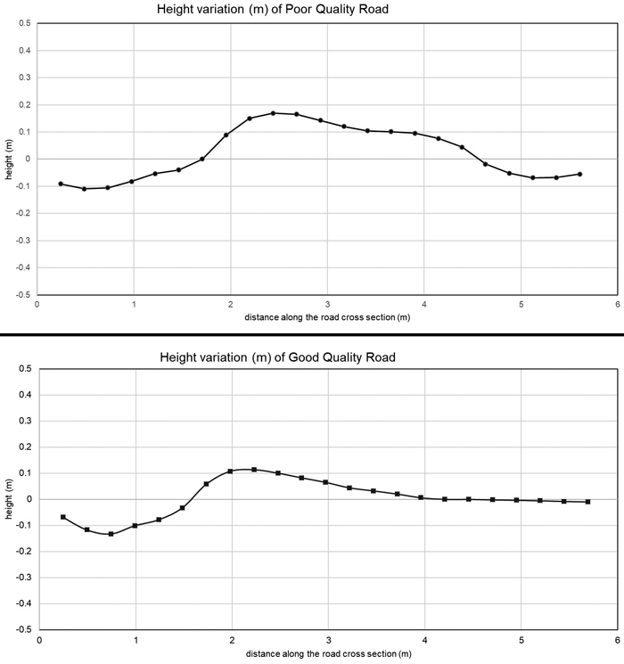
Fig. 2. Cross-sections of bad and good quality roads at 0.25 m resolutions. The Inverse Distance Weighted (IDW) interpolation technique was used to create the surfaces.
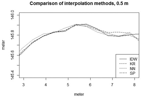
Fig. 3. The interpolation techniques at a resolution of 0.5 metre. In the figure, SP: spline interpolation; KR: kriging interpolation; IDW: inverse distance weighted interpolation; NN: natural neighbour interpolation.
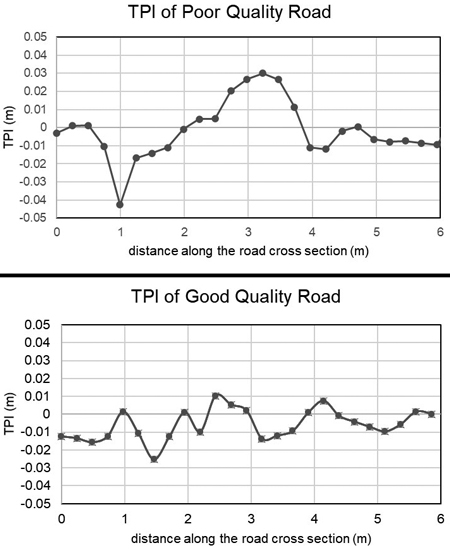
Fig. 4. TPI values for the cross-sections of a bad quality road (up) and good quality road (down). Different interpolations were used at a resolution of 0.25 m. Low pulse density dataset, Tuusniemi. In the figure TPI: Topographic Position Index.
| Table 5. Classification accuracy (%) of TPI index values for structural condition assessments with the reference DEM interpolated with the indicated methods. Tuusniemi, high pulse density laser scanning data at a resolution of 0.5 m, verified against the field data. In the table, SP: spline interpolation; KR: kriging interpolation; IDW: inverse distance-weighted interpolation; NN: natural neighbour interpolation; TPI: Topographic Position Index. | ||||||
| Interpolation technique for reference DEM for TPI index | 3 quality classes | 2 quality classes (poor vs. non-poor) | p-value | |||
| Correctly classified roads | McNemar test (χ2) | Correctly classified roads | McNemar test (χ2) | |||
| IDW | IDW | 11% | 35.315 | 24% | 35.000 | <0.0001 |
| IDW | KR | 13% | 35.268 | 26% | 34.000 | <0.0001 |
| IDW | NN | 24% | 26.894 | 37% | 21.552 | <0.0001 |
| IDW | SP | 22% | 31.091 | 33% | 31.000 | <0.0001 |
| KR | IDW | 17% | 33.084 | 28% | 33.000 | <0.0001 |
| KR | KR | 20% | 32.084 | 30% | 32.000 | <0.0001 |
| KR | NN | 24% | 29.571 | 35% | 26.133 | <0.0001 |
| KR | SP | 7% | 35.121 | 28% | 33.000 | <0.0001 |
| NN | IDW | 17% | 33.084 | 28% | 33.000 | <0.0001 |
| NN | KR | 9% | 34.274 | 26% | 34.000 | <0.0001 |
| NN | NN | 26% | 25.256 | 57% | 16.200 | <0.0001 |
| NN | SP | 15% | 32.077 | 30% | 32.000 | <0.0001 |
| SP | IDW | 57% | 3.806 | 85% | 3.571 | 0.125 |
| SP | KR | 57% | 3.806 | 85% | 3.571 | 0.125 |
| SP | NN | 39% | 26.000 | 70% | 10.286 | 0.002 |
| SP | SP | 57% | 3.806 | 85% | 3.571 | 0.125 |
| Table 6. Class means and standard deviations (SD) of the observations in each quality class for the variables which define good quality classes. In the table, dz: distance of height values from reference DEM; SP: spline interpolation; KR: kriging interpolation; IDW: inverse distance-weighted interpolation; NN: natural neighbour interpolation; TPI: Topographic Position Index. | |||||||||
| Variables | Interpolation technique | Poor class | Satisfactory class | Good class | p-value | McNemar test (χ2) | |||
| mean | SD | mean | SD | mean | SD | ||||
| (sum dz)^2 | SP | 149857.2 | 259466.2 | 49651.9 | 107136.8 | 49262.7 | 128945.5 | 0.887 | 6.444 |
| dz^2 | SP | 24978.0 | 43243.0 | 8786.3 | 18431.0 | 8044.1 | 19625.9 | 0.887 | 6.444 |
| dz | SP | 227.0 | 384.1 | 99.3 | 199.5 | 80.7 | 206.8 | 0.887 | 6.444 |
| mean (dz) | SP | 37.9 | 63.9 | 19.4 | 37.0 | 14.1 | 33.5 | 0.887 | 6.444 |
| mean (dz^2) | SP | 4163.3 | 7206.9 | 1749.2 | 3485.7 | 1332.2 | 3146.9 | 0.887 | 6.444 |
| (sum dz)^2 | NN | 0.1 | 0.2 | 17.6 | 42.1 | 47.2 | 229.0 | 0.887 | 6.444 |
| mean (dz) | NN | 0.0 | 0.1 | 0.0 | 0.1 | –0.1 | 0.3 | 0.669 | 1.145 |
| sum(dz)^2 | IDW | 0.0 | 0.0 | 0.2 | 0.4 | 85.9 | 471.2 | 0.669 | 1.145 |
| TPI using IDW | SP | 0.3 | 1.0 | 0.0 | 1.1 | –0.3 | 0.8 | 0.073 | 1.857 |
| TPI using KR | SP | 0.3 | 1.5 | –0.4 | 1.3 | –0.1 | 0.6 | 0.073 | 1.857 |
| TPI using SP | SP | 0.3 | 1.4 | –0.5 | 1.4 | –0.1 | 0.6 | 0.235 | 2.066 |
| Table 7. Forest road quality classification results of the analysed road sections using weighted distance from the Spline reference DEM with a 3 cm threshold and verified against field observations of structural condition. Overall accuracy: 62.5% Kappa = 0.214. | |||||
| Field measured classes | Classified as... | Classification overall | Producer accuracy (Precision) | ||
| Poor | Satisfactory | Good | |||
| Poor | 2 | 0 | 1 | 3 | 66.66% |
| Satisfactory | 2 | 2 | 5 | 9 | 22.22% |
| Good | 2 | 5 | 21 | 28 | 75.00% |
| Truth Overall | 6 | 7 | 27 | 40 | |
| User Accuracy | 33.33% | 28.57% | 77.77% | ||
| Table 8. Overall classification results for low resolution ALS area after the two-step identification of good and poor classes in terms of structural condition. Overall accuracy: 67.5% Kappa = 0.296 | |||||
| Field measured classes | Classified as... | Classification overall | Producer accuracy (Precision) | ||
| Poor | Satisfactory | Good | |||
| Poor | 2 | 0 | 1 | 3 | 66.66% |
| Satisfactory | 0 | 4 | 5 | 9 | 44.44% |
| Good | 0 | 7 | 21 | 28 | 75.00% |
| Truth Overall | 2 | 11 | 27 | 40 | |
| User Accuracy | 100.00% | 36.36% | 77.77% | ||