| Table 1. The gross vehicle weights, number of axles, and truck and trailer models of the combination vehicles in the study. | ||||
| Truck | Gross vehicle weight (t) | Axles (truck + trailer) | Brand and model, truck | Brand and model, trailer |
| 68_1 | 68 | 3 + 5 | Scania R 650 | Feber Intercars 42P0D6 |
| 68_2 | 68 | 3 + 5 | Scania R 560 | Feber Intercars 42P0D6 |
| 76_1 | 76 | 4 + 5 | Scania R 580 | Närko D4HS11T11 |
| 76_2 | 76 | 4 + 5 | Scania R 580 | Närko D4HS11T11 |
| 76_3 | 76 | 4 + 5 | Scania R 580 | Närko D4HS11T11 |
| 76_4 | 76 | 4 + 5 | Scania R 580 | Närko D4HS11T11 |
| 76_5 | 76 | 4 + 5 | Scania R 730 | Jyki V52-t0 |
| 76_6 | 76 | 4 + 5 | Scania R 730 | Weckman |
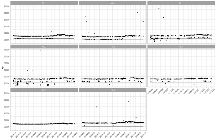
Fig. 1. Tare weight measurements of eight timber trucks over a year. The horizontal lines represent the tare weights in the national transport register (excluding the weight of a loader and other accessories). View larger in new window/tab.
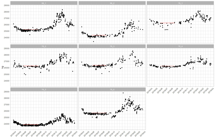
Fig. 2. Filtered tare weights of eight timber trucks over a year. The red lines indicate the normal tare, i.e., the 95th percentile of the tare measurements in summertime. View larger in new window/tab.
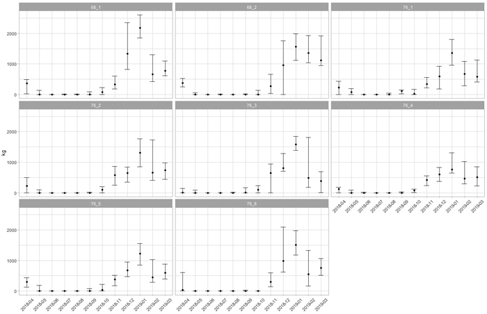
Fig. 3. Monthly median loss of payload of eight timber trucks over a year. The error bars indicate the 10th and 90th percentiles. View larger in new window/tab.
| Table 2. Equivalent annual loss of transport payload due to increased winter tare weight. | ||||||
| Truck id | Gross vehicle weight (kg) | Normal tare (kg) | Maximum payload (kg) | Annual loss of payload (kg) | Annual loss in payloads | Total loads per year in the study |
| 68_1 | 68 000 | 25 359 | 42 641 | 209 740 | 4.9 | 338 |
| 68_2 | 68 000 | 24 459 | 43 541 | 90 000 | 2.1 | 188 |
| 76_1 | 76 000 | 26 305 | 49 695 | 84 718 | 1.7 | 163 |
| 76_2 | 76 000 | 26 314 | 49 686 | 101 100 | 2.0 | 217 |
| 76_3 | 76 000 | 26 422 | 49 578 | 54 260 | 1.1 | 225 |
| 76_4 | 76 000 | 26 321 | 49 679 | 60 960 | 1.2 | 207 |
| 76_5 | 76 000 | 23 940 | 52 060 | 168 300 | 3.2 | 588 |
| 76_6 | 76 000 | 25 722 | 50 278 | 140 580 | 2.8 | 324 |
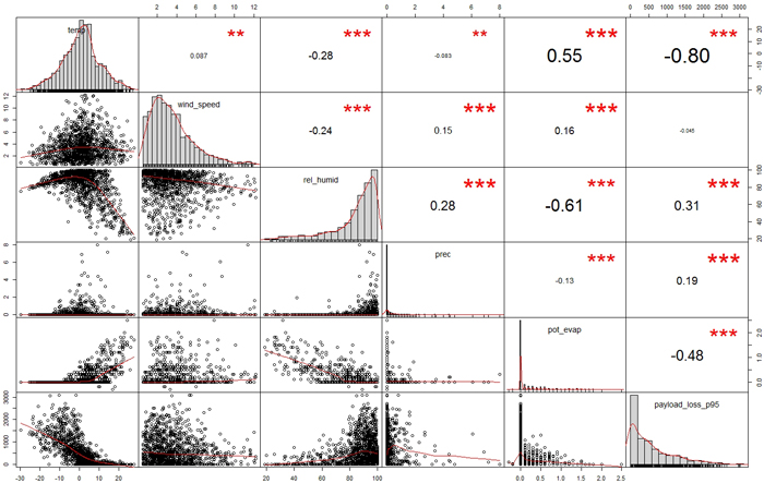
Fig. 4. Spearman correlation factors between payload loss and the weather variables in the training data. The variables (unit in parentheses): temp = momentary temperature (°C), wind_speed = momentary wind speed (m s–1), rel_humid = momentary humidity (%), prec = 3h rainfall (mm), pot_evap = 3h potential evaporation (mm), payload_loss_p95 = potential loss of payload (kg). Significance levels: *** = 0.001, ** = 0.01. View larger in new window/tab.
| Table 3. Model coefficients for logistic regression of probability of no payload loss. | ||||
| Term | Estimate | Standard error | z-score | p-value |
| Intercept | –2.29 | 0.125 | –18.3 | <0.001 |
| Temperature | 0.245 | 0.0153 | 16.1 | <0.001 |
| Table 4. Confusion matrices for the prediction of zero / non-zero payload loss in the training and test data sets. | ||||
| Training data | Test data | |||
| Predicted non-zero payload loss | Predicted zero payload loss | Predicted non-zero payload loss | Predicted zero payload loss | |
| True non-zero payload loss | 949 | 48 | 231 | 16 |
| True zero payload loss | 121 | 178 | 23 | 42 |
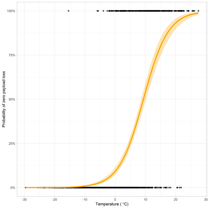
Fig. 5. Probability of zero payload loss as a function of temperature.
| Table 5. Model coefficients of the gamma regression of positive payload loss. Notation a:b means an interaction term between variables a and b. | ||||
| Term | Estimate | Standard error | z-score | p-value |
| Intercept | 4.952 | 0.171 | 28.897 | <0.001 |
| Temperature | 0.033 | 0.020 | 1.635 | 0.102 |
| Relative humidity | 0.014 | 0.002 | 7.357 | <0.001 |
| Precipitation | 0.193 | 0.040 | 4.855 | <0.001 |
| Temperature: Relative humidity | –0.001 | 0.0002 | –5.513 | <0.001 |
| Temperature: Precipitation | –0.026 | 0.006 | –4.476 | <0.001 |
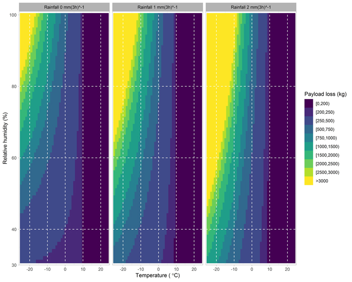
Fig. 6. The model for payload loss as a function of temperature, humidity and rainfall. View larger in new window/tab.