| Table 1. The number of experimental sites in the pre-commercial thinning study according to the age of the stand and early cleaning method (total, point) applied in the site. | ||||||
| Stand age in early cleaning, years | 5 | 6 | 7 | 8 | 10 | |
| Establishment year | 2005 | 2004 | 2003 | 2002 | 2000 | Overall |
| Total cleaning | 4 | 3 | 0 | 1 | 1 | 9 |
| Point cleaning | 3 | 7 | 3 | 0 | 0 | 13 |
| Overall | 7 | 10 | 3 | 1 | 1 | 22 |
| Table 2. The main characteristics of the variables measured in the experimental sites for the pre-commercial thinning (PCT) study in southern Finland (EC = early cleaning, TWI = topographic wetness index). | ||||
| Min | Mean | SD | Max | |
| Site level, n = 22 | ||||
| Site area, ha | 1.8 | 3.5 | 1.5 | 6.9 |
| Density, crop spruces ha–1 | 1150 | 1937 | 342 | 2812 |
| Height of crop spruce, cm | 74 | 129 | 35 | 232 |
| Diameter0.15 of crop spruce, cm | 1.42 | 2.02 | 0.47 | 3.56 |
| Total stand density before EC, trees ha–1 | 10 350 | 22 222 | 11 294 | 59 475 |
| Diameter0.15 of all trees before EC, cm | 0.82 | 1.11 | 0.20 | 1.73 |
| Experimental unit level, n = 132 | ||||
| Experimental unit size, ha | 0.16 | 0.59 | 0.27 | 1.40 |
| Time consumption in EC (recorded), pwh ha–1 | 1.7 | 5.8 | 2.6 | 13.5 |
| Total stand density before EC, trees ha–1 | 5200 | 22 810 | 11 902 | 63 750 |
| Diameter0.15 of all trees before EC, cm | 0.77 | 1.12 | 0.23 | 2.09 |
| Range of elevation change, m | 0.0 | 11.0 | 7.2 | 30.0 |
| Vegetation coverage, % | 0.4 | 9.8 | 7.0 | 38.8 |
| TWI | 5098 | 7018 | 1044 | 10 818 |
| Height growth of removal between EC and PCT, cm year–1 | 18.2 | 37.8 | 9.3 | 62.9 |
| Time consumption in PCT (calculated), twh ha–1 | 4.5 | 11.0 | 4.4 | 26.1 |
| Diameter of removal in PCT, cm | 0.83 | 1.36 | 0.34 | 2.93 |
| Density of removal in PCT, trees ha–1 | 4065 | 18 823 | 12 342 | 65 381 |
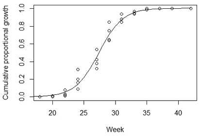
Fig. 1. The cumulative distribution function of the diameter growth of birch within a growing season (line). The function was modeled to estimate the proportion of the growing season that sprouts emerging after early cleaning treatment can still utilize for growth during that year. The initial data (dots) were acquired from Niemistö et al. (2008).
| Table 3. Mixed models (EC1 and EC2) for worktime consumption in early cleaning. EC1 is the primary analysis including removal figures as covariates. The secondary analysis (EC2) replaces the direct figures of removal with its indirect indications, the TWI (topographic wetness index) of a site. The worker effect is redundant in EC2, because it cannot be separated from the site-level variation in the model. The dependent variable is worktime consumption in productive working hours (pwh) ha–1 in both models (N = density, D0.15 = diameter at stump height, EC = early cleaning). All the continuous independent variables are centered around the mean. P-values in bold represent statistically significant differences. | ||||||
| EC1 | EC2 | |||||
| Estimate | Std. Error | P-value | Estimate | Std. Error | P-value | |
| Intercept | 5.303 | 0.509 | <0.001 | 5.343 | 0.554 | <0.001 |
| N before EC, 1000 trees ha–1 | 0.175 | 0.015 | <0.001 | |||
| D0.15 before EC, cm | 1.921 | 0.771 | 0.016 | |||
| Season, ref. Spring | ||||||
| Summer | 1.970 | 0.255 | <0.001 | 1.955 | 0.318 | <0.001 |
| Autumn | 0.939 | 0.261 | <0.001 | 0.884 | 0.317 | 0.006 |
| Ln(Area), ha | –1.545 | 0.345 | <0.001 | –1.731 | 0.453 | <0.001 |
| Elevation change, m | 0.256 | 0.119 | 0.035 | 0.103 | 0.167 | 0.538 |
| EC-method, ref. Total cleaning | ||||||
| Point cleaning | –0.774 | 0.412 | 0.079 | –0.742 | 0.689 | 0.293 |
| Vegetation cover, % | –0.017 | 0.027 | 0.516 | –0.005 | 0.033 | 0.892 |
| Season:Vegetation cover, ref. Spring | ||||||
| Summer:Vegetation cover | 0.086 | 0.037 | 0.024 | 0.107 | 0.047 | 0.025 |
| Autumn:Vegetation cover | 0.057 | 0.038 | 0.138 | 0.004 | 0.047 | 0.939 |
| TWI, in thousands | 0.549 | 0.221 | 0.014 | |||
| Random effects | Variance | Std.Dev. | Variance | Std.Dev. | ||
| Stand:Worker | 0.317 | 0.563 | 2.104 | 1.451 | ||
| Worker | 1.267 | 1.126 | 0.000 | 0.000 | ||
| Residual | 1.381 | 1.175 | 2.081 | 1.443 | ||
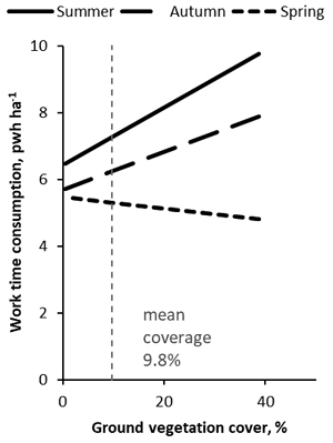
Fig. 2. Estimate of productive worktime consumption in early cleaning in spruce stands according to the EC1 model. Cleanings were applied in different seasons and with varying degrees of ground vegetation coverage. Vegetation cover was determined in the summer or autumn in all treatments, so not necessarily during or close to the application of the treatment. The main effects differed significantly between all seasons. The slope was statistically significant in the summer, but not in the autumn or spring.
| Table 4. Mixed models for worktime consumption (model PCT1, total work hours ha–1), removal of density (model PCTden, Ln[trees ha–1]), and diameter of density (model PCTdiam, cm) in PCT in studied spruce stands (N = density, D0.15 = diameter at stump height). All the continuous independent variables are centered around the mean. P-values in bold represent statistically significant differences. | |||||||||
| PCT1 | PCTden a | PCTdiam | |||||||
| Estimate | Std. Error | P-value | Estimate | Std. Error | P-value | Estimate | Std. Error | P-value | |
| Intercept | 10.698 | 0.521 | <0.001 | 2.940 | 0.102 | <0.001 | 1.368 | 0.062 | <0.001 |
| Season, ref. Spring | |||||||||
| Summer | –1.000 | 0.410 | 0.016 | –0.136 | 0.066 | 0.043 | –0.091 | 0.062 | 0.146 |
| Autumn | –0.291 | 0.421 | 0.490 | –0.014 | 0.069 | 0.839 | –0.112 | 0.064 | 0.082 |
| EC-method, ref. Total cleaning | |||||||||
| Point cleaning b | –1.456 | 0.622 | 0.028 | –0.241 | 0.126 | 0.068 | 0.099 | 0.068 | 0.158 |
| N before EC, 1000 trees ha–1 | 0.200 | 0.023 | <0.001 | 0.041 | 0.004 | <0.001 | –0.012 | 0.003 | <0.001 |
| D0.15 before EC, cm | –1.503 | 1.191 | 0.212 | –0.125 | 0.218 | 0.566 | –0.103 | 0.144 | 0.482 |
| Random effects: | Variance | Std.Dev. | Variance | Std.Dev. | Variance | Std.Dev. | |||
| Stand | 1.244 | 1.116 | 0.007 | 0.086 | 0.007 | 0.086 | |||
| Residual | 3.725 | 1.930 | 0.086 | 0.293 | 0.086 | 0.293 | |||
| a) Log-transformed dependent variable used in PCTden. b) It should be noted that placement of experiment plots differed between EC methods (see discussion). | |||||||||
| Table 5. Mixed model (Hremo) for height growth (cm year–1) of the removal between early cleaning (EC) and pre-commercial thinning (PCT) in spruce stands studied in southern Finland (N = density, D0.15 = diameter at stump height). All the continuous independent variables are centered around the mean. P-values in bold represent statistically significant differences. | |||
| Estimate | Std. Error | P-value | |
| Intercept | 34.190 | 1.814 | <0.001 |
| Season, ref. Spring | |||
| Summer | 0.397 | 0.345 | 0.249 |
| Autumn | 7.669 | 0.361 | <0.001 |
| EC-method, ref. Total cleaning | |||
| Point cleaning | 2.554 | 2.338 | 0.286 |
| Species, ref. Downy birch | |||
| Conifer | –1.417 | 0.544 | 0.009 |
| Silver birch | 0.432 | 0.461 | 0.349 |
| Aspen | –5.966 | 1.015 | <0.001 |
| Other | 7.850 | 2.571 | 0.002 |
| Sorbus | –2.025 | 0.438 | <0.001 |
| Salix | –1.795 | 0.615 | 0.004 |
| N before EC, 1000 trees ha–1 | –0.142 | 0.033 | <0.001 |
| D0.15 before EC, cm | 2.367 | 1.514 | 0.118 |
| Random effects: | Variance | Std.Dev. | |
| Stand | 28.350 | 5.324 | |
| Residual | 38.110 | 6.173 | |
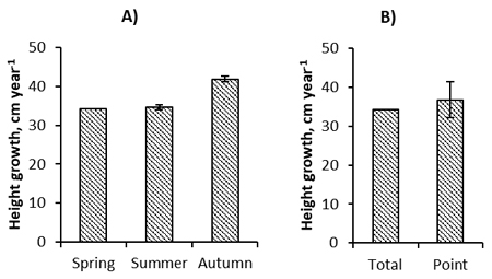
Fig. 3. Post early cleaning (EC) growth rate of the trees removed in pre-commercial thinning (mainly resprouts from EC) according to the season of application (A) or the method (B) of EC in the studied spruce stands. The error bars are the 95% confidence intervals of the parameter estimates compared to the reference category (Spring in A or Total in B) in the Hremo model.
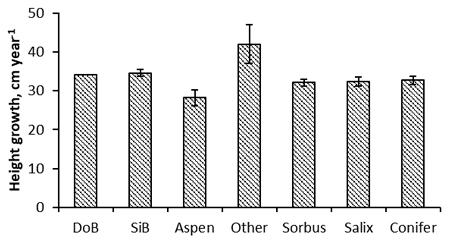
Fig. 4. Post early cleaning growth rate of the trees of different species removed in pre-commercial thinning (mainly resprouts from EC) of the studied spruce stands (DoB = downy birch, SiB = silver birch). The error bars are the 95% confidence intervals of the parameter estimates compared to the reference category (DoB) in the Hremo model.
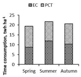
Fig. 5. The effect of the season of application of early cleaning (EC) on the time consumption of the juvenile stand management program in total working hours (twh) ha–1, i.e. on the combined time consumption of EC and 4–5 growing seasons later following pre-commercial thinning (PCT).
| Table 6. Costs of early cleaning (EC) and pre-commercial thinning (PCT) with a nominal rate (0%) and with a 3% discounted rate in totally cleaned and point cleaned spruce stands when cleaning was applied in the spring, summer, or autumn. The present values have been calculated to the timepoint when the first EC treatment was applied in the spring. | |||||
| EC, € ha–1 | PCT, € ha–1 | Overall, € ha–1 | EC time, years | PCT time, years | |
| Nominal rate, 0% | |||||
| Spring - Total | 266 | 326 | 592 | ||
| Summer - Total | 365 | 295 | 661 | ||
| Autumn - Total | 313 | 317 | 630 | ||
| Discount rate, 3% | |||||
| Spring - Total | 266 | 312 | 578 | 0.00 | 4.40 |
| Summer - Total | 365 | 283 | 647 | 0.14 | 4.40 |
| Autumn - Total | 312 | 303 | 615 | 0.39 | 4.40 |