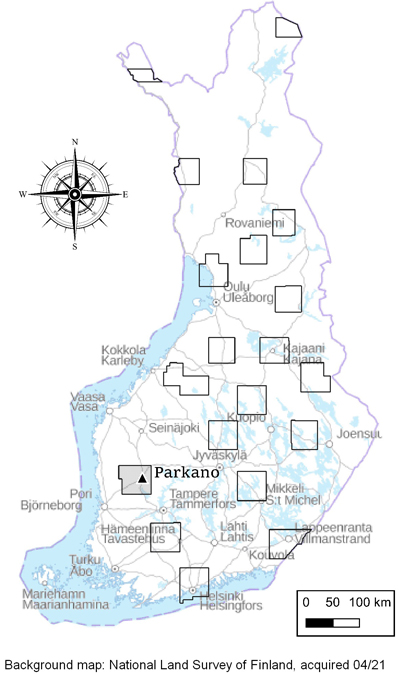
Fig. 1. The coverage of high-density airborne LiDAR data after inventories in 2020. The study of improving stream extraction and soil wetness mapping by increasing LiDAR data density was implemented in the catchment of lake Kovesjärvi (62°04´N, 22°50´E), which is located in Parkano municipality, roughly 240 km northwest of Helsinki, Finland.
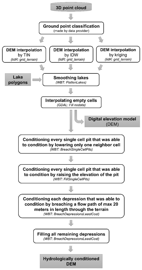
Fig. 2. Workflow of generating a hydrologically conditioned DEM from a LiDAR-derived 3D point cloud. DEM conditioning was an essential part of this study of developing overland flow routing routines by using increased LiDAR data density. Three alternative interpolation methods were tested for DEM processing. The aim is to remove local sinks and depressions that prevent continuous modeling of overland water flow: pits are defined as single cells without any downsloping neighbor and depressions as larger bowl-like features without a downslope direction. Pits and depressions may be artefacts or real, but in any case they need to be either filled or breached for creating a hydrologically conditioned DEM. The open-source tools that were used in the study are named in parenthesis. TIN = Triangulated Irregular Network. IDW = Inverse-distance Weighting. lidR = R package for airborne LiDAR data manipulation and visualization for forestry applications, Version 3.1.2. WBT = WhiteboxTools, Version 1.4.0. GDAL = Geospatial Data Abstraction Library.
| Table 1. Comparison of LiDAR data point densities, DEM cell sizes, and interpolation methods in overland flow routing, which are the main results of this study aiming at improved stream extraction and soil wetness mapping within a forested catchment. In general, breaching leads to more realistic flow paths than filling, and the changes in DEM are smaller on average with breaching. The more overlapping stream/ditch segments were found in the stream extraction, the better flow routing corresponds to the topographical database maintained by the NLS (2021b). However, raster cell may affect flow accumulation, thus the overlaps should not be compared with different cell sizes. Key flow paths were selected so that they were located along the main waterways and were divided roughly evenly within the catchment. | ||||||||||||
| Low-density airborne LiDAR | High-density airborne LiDAR | |||||||||||
| DEM cell size | 1 m | 2 m | 1 m | 2 m | ||||||||
| Interpolation method | TIN | IDW | Kriging | TIN | IDW | Kriging | TIN | IDW | Kriging | TIN | IDW | Kriging |
| Share of remodeled raster cells in conditioned DEM: | ||||||||||||
| Breached cells (>10 cm) | 1.4% | 1.1% | 1.1% | 4.6% | 3.1% | 4.5% | 3.9 % | 3.1% | 3.9% | 6.3% | 5.8% | 6.6% |
| Mean breach depth [m] | –0.18 | –0.11 | –0.12 | –0.14 | –0.13 | –0.14 | –0.12 | –0.11 | –0.12 | –0.16 | –0.16 | –0.17 |
| Filled cells (>10 cm) | 6.0% | 5.9% | 4.9% | 5.8% | 5.6% | 5.1% | 3.4% | 5.6% | 2.8% | 6.4% | 5.6% | 4.0% |
| Mean filling height [m] | 0.62 | 0.51 | 0.43 | 0.45 | 0.48 | 0.37 | 0.53 | 0.46 | 0.44 | 0.52 | 0.55 | 0.35 |
| Overlapped streams/ditches using different channelization thresholds: | ||||||||||||
| 0.1 ha | 73% | 73% | 74% | 70% | 70% | 71% | 76% | 76% | 76% | 72% | 72% | 72% |
| 0.2 ha | 63% | 63% | 64% | 61% | 61% | 62% | 67% | 67% | 67% | 63% | 64% | 64% |
| 0.5 ha | 49% | 50% | 50% | 48% | 48% | 49% | 52% | 53% | 53% | 50% | 50% | 50% |
| 1.0 ha | 38% | 39% | 38% | 37% | 37% | 38% | 39% | 40% | 40% | 38% | 38% | 38% |
| Key flow paths found: | ||||||||||||
| Culverts (n = 20) | 75% | 70% | 75% | 60% | 55% | 60% | 75% | 85% | 85% | 65% | 80% | 85% |
| Streams/ditches (n = 20) | 65% | 55% | 80% | 55% | 70% | 55% | 70% | 85% | 85% | 80% | 90% | 85% |
| Altogether (n = 40) | 70% | 63% | 78% | 58% | 63% | 58% | 73% | 85% | 85% | 73% | 85% | 85% |
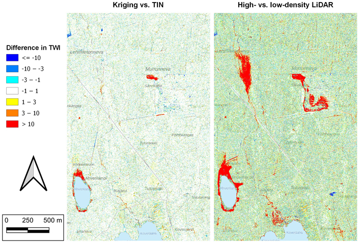
Fig. 3. Comparing the effect of interpolation method (kriging vs. TIN) and LiDAR point density (high vs. low) on Topographic Wetness Index (TWI), which was derived using improved overland flow routing routines developed in this research article. On the left, the difference between TWIs calculated from kriging- and TIN-based elevation models (high-density LiDAR in common). On the right, the respective comparison between high- and low-density LiDAR-derived TWIs (kriging in common). The color scale and symbology are the same in both figures. TWI index was clearly more sensitive to data point density than to interpolation method. Red areas on the right illustrate areas were the TWI computed from low-density LiDAR data was more than 10 units larger than the TWI computed from high-density LiDAR data. For example, the difference is very clear on a mire in the top left, as ditches were poorly recognized by low-density LiDAR, and the whole mire was filled in the DEM conditioning so that continuous flow routing was achieved.