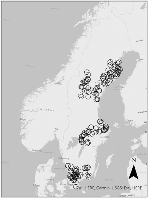
Fig. 1. Inventoried sites included in the analysis (○) in the South (n = 48), Central (n = 45) and North (n = 81) regions in Sweden. © Lantmäteriet.
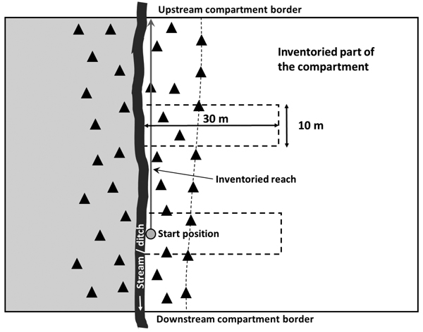
Fig. 2. Schematic illustration of the survey set-up for a compartment traversed by a stream (or ditch) with a forest buffer (the zone between the stream and thin dashed line). The side of the stream hosting the largest part of the harvested compartment was selected (white area). The grey circle shows the start position of the inventory and the attached arrow shows the inventoried reach, i.e. the longest distance from the start position to the upstream or downstream compartment border. In this example, the longest distance was to the upstream border and the distance to be inventoried was 30–99 m, requiring an inventory of two plots (indicated by dashed rectangles).
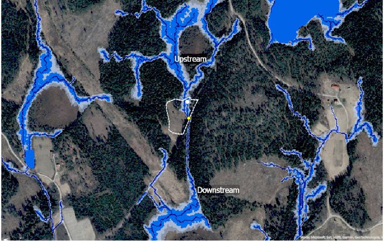
Fig. 3. Aerial photo of a compartment (dotted white line) traversed by a stream, including the up- and downstream reaches which were used for assessing the stream type. In this case, the up- and downstream reaches were classified as ‘natural’ from the map and the inventoried reach (i.e., the reach between the white and yellow circles) was categorized as ‘modified’ during the field inventory, giving the stream type ‘modified stream’. The photo is overlaid by the depth-to-water map obtained from Swedish Forest Agency (https://www.skogsstyrelsen.se/). © Lantmäteriet.
| Table 1. Inventory protocol for the forest buffer and site characteristics presented in this study including the inventoried variables, their available classes or measure and comments on the methods or classes used (see also Ring et al. 2020). | ||
| Variable | Available classes or measure | Comments |
| Character of water reach bordering the compartment | Natural stream | Assessed for the water reach traversing or bordering the compartment. A natural stream is one showing no evidence of human interference. |
| Modified stream | Modified stream: signs of human activity, for example straightened or deepened stream channel. | |
| Ditch | ||
| Lake | ||
| Wide river | ||
| Other | ||
| Inventoried shore length | Meters | Measured using a tablet computer from the start position to the border of the compartment, or end of the reach if it ends before the compartment border (determined by eye from the start position), using ’Collector for ArcGIS’ with Esri´s basemap for Sweden, based on Lantmäteriet´s open data (orthophoto), as background. |
| Channel width | Meters without decimal fractions | The channel width at the start position estimated by eye. Stream: width of stream bed with exposed mineral soil or where the vegetation shows signs of high water levels. Ditch: width at the soil surface. |
| Shoreline coverage of the forest buffer | 100% | Percentage class of the shoreline forest buffer coverage, i.e., coherent area with trees (with breast-height diameter >7 cm) spaced <10 m apart, along the entire inventoried reach. |
| 75–100% | ||
| 50–75% | ||
| <50% | ||
| No buffer | ||
| Width of forest buffer | Meters without decimal fractions | The width from the most distant tree trunk to the shoreline within the plot stepped out or assessed by eye. |
| Canopy structure of the forest buffer | Multi-layered | Canopy structure of the buffer along the entire inventoried reach. |
| Single-layered | ||
| Single trees | ||
| Shrubs | ||
| Wetland forest | ||
| Soil moisture class | 1–4 | Dry (1), mesic (2), moist (3) or wet (4). The soil moisture class determined for the first 10 m from the shoreline of the plots. |
| Surface structure class | 1–5 | Even ground (class 1) to technically impossible to harvest (class 5), determined for the plots. |
| Trafficability class | 1–5 | Very good (class 1), allowing forestry work year-round to very bad (class 5) restricting forestry work to periods with frozen ground, according to Berg (2006), determined for the plots. |
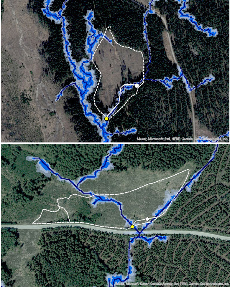
Fig. 4. Aerial photos of two inventoried sites, representing the stream types ‘natural stream’ (top) and ‘ditch’ (bottom), overlaid by the depth-to-water map obtained from the Swedish Forest Agency (https://www.skogsstyrelsen.se/). The dotted white lines indicate compartment boundaries and the solid white lines the randomly selected water reaches (obtained from the vector layer of hydrography, https://www.lantmateriet.se). White circles indicate start positions and yellow circles the end of the inventoried reaches. © Lantmäteriet.
| Table 2. Information regarding the compartment selection, number of inventoried plots, compartment soil characteristics, surveyed shore lengths, channel widths and number of inventoried lake, stream and ditch reaches (or stream types). The data were collected for three regions (South, Central and North) in Sweden and are presented per region and in total. ‘Mean’ denotes the arithmetic mean and ‘SE’ the sample standard error. | ||||
| South region | Central region | North region | Total | |
| No. of visited compartments | 104 | 93 | 135 | 332 |
| No. of surveyed compartments | 48 | 45 | 81a | 174 |
| No. of unsurveyed compartments | 56 | 48 | 54 | 158 |
| Reason for not surveying: | ||||
| – not site-prepared | 46 | 22 | 31 | 99 |
| – could not be reached | 7 | 16 | 16 | 39 |
| – lacked a water body | 1 | 0 | 2 | 3 |
| – other | 1 | 9 | 4 | 14 |
| – no reason stated | 1 | 1 | 1 | 3 |
| All data presented below refer to compartments included in the analysis | ||||
| No. of inventoried plots per compartment: | ||||
| Mean | 3.3 | 2.8 | 2.6 | 2.9 |
| Min–max | 2–5 | 2–4 | 1–4 | 1–5 |
| No. of inventoried plots in total | 157 | 125 | 214 | 496 |
| Size of surveyed harvested compartments: | ||||
| Mean (ha) | 3.5 | 6.7 | 9.1 | 6.9 |
| Min–max (ha) | 0.2–11.9 | 0.7–40.2 | 0.6–45.2 | 0.2–45.2 |
| Trafficability classb– mean (SE) | 2.4 (0.1) | 2.6 (0.1) | 2.5 (0.1) | 2.5 (0.07) |
| Surface structure classb– mean (SE) | 1.6 (0.08) | 1.6 (0.07) | 1.4 (0.07) | 1.5 (0.04) |
| Soil moisture classb,c– mean (SE) | 2.4 (0.06) | 2.4 (0.09) | 2.9 (0.06) | 2.6 (0.04) |
| Surveyed shore length: | ||||
| Mean (m) | 105 | 143 | 122 | 123 |
| Min–max (m) | 23–500 | 50–470 | 20–480 | 20–500 |
| Total (km) | 5.0 | 6.4 | 9.9 | 21.3 |
| Channel width (at the start position) for streams and ditches: | ||||
| Mean (m) | 2.1 | 1.8 | 3.2 (2.1)d | 2.5 (2.0)d |
| Min–max (m) | 1–7 | 1–4 | 0–80 (0–6)d | 0–80 (0–7)d |
| Type of water, no. per category (reach class / stream type): | ||||
| Natural stream | 6 / 3 | 5 / 3 | 39 / 23 | 50 / 29 |
| Modified stream | 9 / 25 | 9 / 26 | 3 / 43 | 21 / 94 |
| Ditch | 27 / 14 | 28 / 13 | 32 / 8 | 87 / 35 |
| Lake | 6 | 3 | 7 | 16 |
| a Including two compartments compartments which had not been site-prepared but had all relevant data. b See Table 1 for definitions of classes. c Determined for the first 10 m from the shoreline of the plots. d Value when the 80-m wide river was excluded. | ||||
| Table 3. Results from the statistical analyses according to Models 1 and 2 using the GENMOD procedure in SAS software. The denominator degrees of freedom were 3 for reach class and stream type, 2 for region and 6 for the interaction between reach class (or stream type) and region, except for channel width with 2 degrees of freedom for reach class (or stream type) and 4 degrees of freedom for the interaction with region. Effects were regarded statistically significant if p < 0.05. | ||||||
| Dependent variable | Factor | Chi-square statistics | p-value | Factor | Chi-square statistics | p-value |
| Model 1 | ||||||
| Forest buffer width | Reach class | 37.5 | <0.01 | Stream type | 30.1 | <0.01 |
| Region | 0.10 | 0.95 | Region | 0.1 | 0.93 | |
| Reach class × Region | 2.0 | 0.92 | Stream type × Region | 1.6 | 0.95 | |
| Inventoried shore length | Reach class | 7.2 | 0.066 | Stream type | 2.1 | 0.56 |
| Region | 2.6 | 0.27 | Region | 3.3 | 0.19 | |
| Reach class × Region | 2.8 | 0.83 | 2.6 | 0.86 | ||
| Channel width | Reach class | 0.3 | 0.84 | Stream type | 0.5 | 0.79 |
| Region | 0.03 | 0.98 | Region | 0.9 | 0.64 | |
| Reach class × Region | 0.1 | 1.0 | Stream type × Region | 0.2 | 0.99 | |
| Size of harvested area | Reach class | 0.5 | 0.93 | Stream type | 0.3 | 0.96 |
| Region | 0.8 | 0.67 | Region | 6.6 | 0.036 | |
| Reach class × Region | 13.4 | 0.037 | Stream type × Region | 11.3 | 0.078 | |
| No. of plots per compartment | Reach class | 5.3 | 0.15 | Stream type | 2.3 | 0.52 |
| Region | 13.7 | <0.01 | Region | 7.9 | 0.020 | |
| Reach class × Region | 4.2 | 0.65 | Stream type × Region | 3.2 | 0.79 | |
| Model 2 | ||||||
| Forest buffer width | Reach class | 78.9 | <0.01 | Stream type | 60.4 | <0.01 |
| Region | 0.4 | 0.83 | Region | 0.05 | 0.98 | |
| Inventoried shore length | Reach class | 6.0 | 0.11 | Stream type | 1.6 | 0.65 |
| Region | 3.8 | 0.15 | Region | 4.0 | 0.14 | |
| Channel width | Reach class | 1.2 | 0.55 | Stream type | 3.3 | 0.19 |
| Region | 0.4 | 0.83 | Region | 0.8 | 0.66 | |
| No. of plots per compartment | Reach class | 5.7 | 0.13 | Stream type | 1.6 | 0.65 |
| Region | 19.3 | <0.01 | Region | 16.4 | <0.01 | |
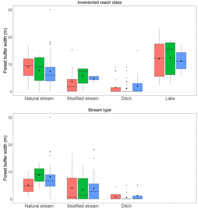
Fig. 5. Boxplots of forest buffer width for the South (red), Central (green) and North (blue) regions in Sweden by reach class (above) and stream type (below), based on compartment means. Boxes show the 25% and 75% percentiles, with a thick horizontal line and diamond indicating the median and arithmetic mean, respectively. The vertical bars show the minimum and maximum values unless observations deviate by more than 1.5 times the interquartile range (i.e., the difference between the 75th and 25th percentiles). In such cases, these observations are indicated with points.
| Table 4. Mean widths of forest buffers for the indicated classes of inventoried reaches in the South, Central, and North regions of Sweden and for all regions together, calculated by the least squares mean method using Models 1 and 2. The last two columns show the proportion lacking a forest buffer and the proportion containing buffer covering 100% of the surveyed reach for all three regions together. Mean = least squares mean calculated using the GENMOD procedure in SAS software, SE = standard error calculated using the GENMOD procedure and re-transformed from logarithmic values using the delta method, n = sample size | ||||||
| Inventoried reach class | Forest buffer width (m) | Proportion lacking a buffer (%) | Proportion with 100% shoreline coverage (%) | |||
| Mean (SE) | ||||||
| n | ||||||
| Southa | Centrala | Northa | All regionsb | All regions | All regions | |
| Natural stream | 9.0 (1.8) | 7.8 (2.0) | 7.3 (0.7) | 7.9 (0.8) | 12c | 64c |
| 6 | 5 | 39 | 50 | |||
| Modified stream | 3.7 (1.5) | 5.7 (1.5) | 4.7 (2.6) | 4.6 (1.0) | 19 | 33 |
| 9 | 9 | 3 | 21 | |||
| Natural and modified streams | 5.8 (1.2) | 6.4 (1.2) | 7.2 (0.7) | 6.6 (0.6) | 14c | 55c |
| 15 | 14 | 42 | 71 | |||
| Ditch | 1.4 (0.9) | 1.1 (0.8) | 2.0 (0.8) | 1.5 (0.5) | 61c | 10c |
| 27 | 28 | 32d | 87d | |||
| Lake | 12.1 (1.8) | 12.4 (2.6) | 11.4 (1.7) | 12.0 (1.1) | 0 | 100 |
| 6 | 3 | 7 | 16 | |||
| a Least squares means and SE were calculated using Model 1. b Least squares means and SE were calculated using Model 2. c nna = 1 (for shoreline coverage) corresponding to 1–2% of the sample. d nna = 1. | ||||||
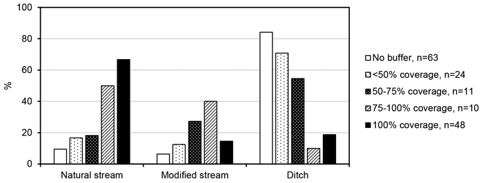
Fig. 6. Proportions of inventoried reaches in the forest buffer shoreline coverage classes no buffer, <50% coverage, 50–75% coverage, 75–100% coverage and 100% coverage (nna = 2). ‘n’ indicates the number of observations in each class.