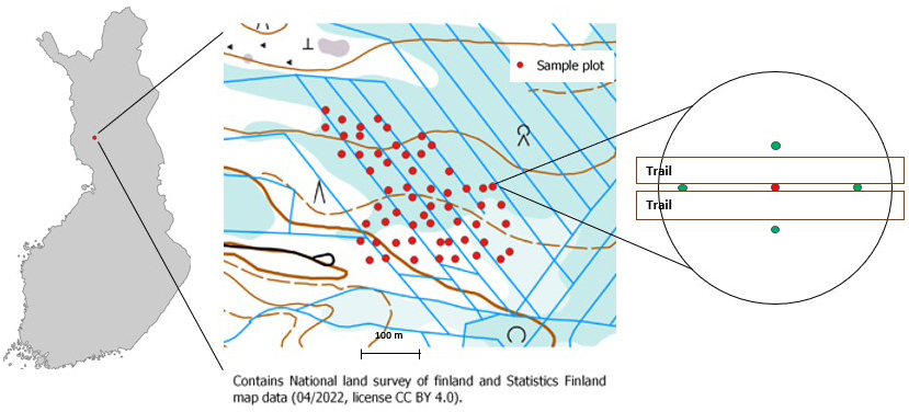
Fig. 1. Map of Finland showing the location of the research site where the sample plots were established on the drained peatland forest (ETRS-TM35FIN 7368023,425587). On the sample plot (radius: 9 m), the red dot in the middle of the strip road is the centre of the plot and the excavation by which the peat type, the degree of peat decomposition and the mineral soil type were identified. The water level was measured weekly. The green dots are the measurement points for the thickness of the peat layer; the thickness measurement was also performed from the centre of the plot.
| Table 1. Total precipitation and mean air temperature for June to August in 2017 and 2019 and long-term averages (2000–2019). The data for Hirvas have been calculated using the kriging interpolation method. |
| Month, Annual | June | July | August | Annual |
| Precipitation (mm) |
| Hirvas 2017 | 56 | 81 | 54 | 490 |
| Hirvas 2019 | 86 | 14 | 97 | 572 |
| Rovaniemi 2000–2019 | 64 (19–125) | 79 (15–152) | 70 (7–178) | 639 (422–874) |
| Temperature (°C) |
| Hirvas 2017 | 11.8 | 15.6 | 12.8 | 1.7 |
| Hirvas 2019 | 13.7 | 14.8 | 13.4 | 1.6 |
| Rovaniemi 2000–2019 | 12.5 | 16.1 | 13.4 | 1.8 |
| Table 2. Thickness of peat layer, volume of stand, depth of ditch and degree of decomposition of peat according to the type of mineral soil under the peat layer. The soil types are saSi = clay silt, siHkMr = silt sandy moraine, HkMr = sand moraine, srHkMr = gravel sand moraine, Hk = sand. |
| Soil | N | Peat layer, cm | Volume of stand, m3 ha–1 | Depth of ditch, cm | Degree of decomposition of peat |
| Mean | Min | Max | Mean | Min | Max | Mean | Min | Max | Mean | Min | Max |
| saSi | 5 | 49 | 41 | 57 | 102 | 45 | 174 | 28 | 23 | 34 | 4.0 | 2 | 7 |
| siHkMr | 12 | 42 | 23 | 70 | 110 | 40 | 181 | 36 | 20 | 44 | 4.7(10) | 3 | 7 |
| HkMr | 25 | 40 | 27 | 70 | 108 | 11 | 181 | 40 | 19 | 55 | 2.9(22) | 1 | 5 |
| srHkMr | 4 | 38 | 21 | 53 | 85 | 23 | 133 | 42 | 13 | 52 | 2.0 | 2 | 5 |
| Hk | 7 | 38 | 26 | 61 | 92 | 55 | 158 | 42 | 18 | 56 | 3.0 | 2 | 5 |
| Table 3. The average groundwater levels (in cm) on measurement days according to soil types in 2017 and 2019. Precipitation is the sum of the precipitation in the week preceding the measurement. The soil types are saSi = clay silt, siHkMr = silt sandy moraine, HkMr = sand moraine, srHkMr = gravel sand moraine, Hk = sand. |
| Year 2017 |
| Soil | Group | N | 28. June | 6. July | 12. July | 20. July | 27. July | 3. Aug | 10. Aug | 16. Aug |
| saSi | Silty | 5 | 14 | 14 | 18 | 13 | 20 | 20 | 26 | 28 |
| siHkMr | Silty | 12 | 15 | 16 | 25 | 16 | 26 | 28 | 36 | 39 |
| HkMr | Sandy | 25 | 18 | 19 | 36 | 20 | 36 | 38 | 44 | 46 |
| srHkMr | Sandy | 4 | 16 | 16 | 27 | 18 | 27 | 27 | 36 | 34 |
| Hk | Sandy | 7 | 20 | 23 | 36 | 24 | 36 | 38 | 43 | 41 |
| Rain, mm | | 29 | 26 | 5 | 34 | 5 | 22 | 10 | 12 |
| Year 2019 |
| Soil | Group | N | 19. June | 26. June | 3. July | 10. July | 17. July | | | |
| saSi | Silty | 5 | 18 | 14 | 18 | 21 | 27 | | | |
| siHkMr | Silty | 11 | 17 | 14 | 19 | 24 | 34 | | | |
| HkMr | Sandy | 25 | 28 | 19 | 30 | 37 | 47 | | | |
| srHkMr | Sandy | 3 | 22 | 16 | 22 | 26 | 38 | | | |
| Hk | Sandy | 7 | 28 | 23 | 31 | 36 | 44 | | | |
| Rain, (mm) | | 19 | 37 | 11 | 6 | 4 | | | |
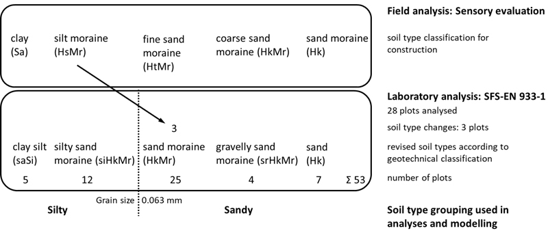
Fig. 2. Soil sample analyses and classification. First, a sensory evaluation (RT) was made in the field for all 53 plots. Second, for control purposes, 28 samples from the important groups of silt moraine and fine sand moraine were further analysed in the laboratory. This was done to ensure that the demarcation of samples between Silty and Sandy groups was correct in further analyses. Three soil samples were redirected over the critical demarcation line (grain size: 0.063 mm). Finally, soil samples were placed into revised soil types (GEO), which were further divided into Silty and Sandy groups using the Mann–Whitney U-test.
| Table 4. Tested explanatory variables for the linear mixed effects model. The parameters of distributions (continuous variables) or the frequencies (numbers of observations in the longitudinal data) and the proportions of the categories (categorical variables) are presented in the table. |
| Variable | Mean | Median | Minimum | Maximum |
| Continuous variables: |
| Groundwater level, cm (response) | 27.35 | 24.00 | 8.00 | 65.00 |
| Volume of stock, m3 ha–1 | 108.20 | 111.60 | 10.50 | 181.00 |
| Measurement, nr. | 3.93 | 4.00 | 1.00 | 8.00 |
| Rainfall (during week), mm | 16.89 | 12.00 | 3.70 | 37.20 |
| Temperature (during day), °C | 14.04 | 13.90 | 10.20 | 16.90 |
| Peat decomposition, scale 1–8 | 3.34 | 3.00 | 1.00 | 7.00 |
| Altitude, m a.s.l. | 83.02 | 82.83 | 80.40 | 86.64 |
| Ditch depth, cm | 35.82 | 35.00 | 13.00 | 56.00 |
| Depth of peat layer, cm | 41.44 | 39.00 | 21.00 | 70.00 |
| Categorical variables: |
| Peat type | wooden-sphagnum peat: 85% (515), wooden-carex peat 15% (91) |
| Mineral soil type | Silty: 31% (190), Sandy: 69% (416) |
| Table 5. Parameter estimates and tests of a general linear mixed effects model (Gaussian) for the groundwater level. Std. err. denotes the standard error of the estimates, df denotes the degrees of freedom, t-values are the test values for the parameter estimates, and p is the statistical significance level. R2 for the marginal model was 68.4% and that for the conditional model was 81.4%. |
| Variable | Coefficient | Std. err. | df | t-value | p |
| Fixed effects: |
| Intercept | 13.791 | 4.905 | 511.000 | 2.812 | 0.005 |
| Peat type, carex-sphagnum peat, ref. wooden-carex peat | –0.155 | 0.064 | 83.000 | –2.412 | 0.018 |
| Volume of timber stock, m3 ha–1 | 0.002 | 0.001 | 83.000 | 2.973 | 0.004 |
| Rainfall (during the period week), mm | –0.014 | 0.001 | 511.000 | –26.370 | 0.000 |
| Measurement, nr | 0.083 | 0.005 | 511.000 | 16.044 | 0.000 |
| Mineral soil type, sandy, ref. silty | 1.110 | 0.233 | 83.000 | 4.761 | 0.000 |
| Depth of peat layer, cm | –0.367 | 0.134 | 83.000 | –2.748 | 0.007 |
| Ditch depth, cm | 0.003 | 0.002 | 83.000 | 1.928 | 0.057 |
| Altitude, m.o.s.l. | –0.133 | 0.060 | 83.000 | –2.220 | 0.029 |
| Mineral soil type*Depth of peat layer | –0.025 | 0.006 | 83.000 | –4.105 | 0.000 |
| Depth of peat layer*Altitude | 0.004 | 0.002 | 83.000 | 2.713 | 0.008 |
| Random effects (variances) and phi (AR1 correlation structure), 95% confidence limits in the parenthesis: |
| Random year effect | 1.509e-2 (0.079e-2–0.289) |
| Random sample point effect | 1.354e-2 (0.593e-2–3.092e-2) |
| Residual | 4.092e-2 (3.206e-2–5.223e-2) |
| Phi | 0.511 (0.377–0.623) |
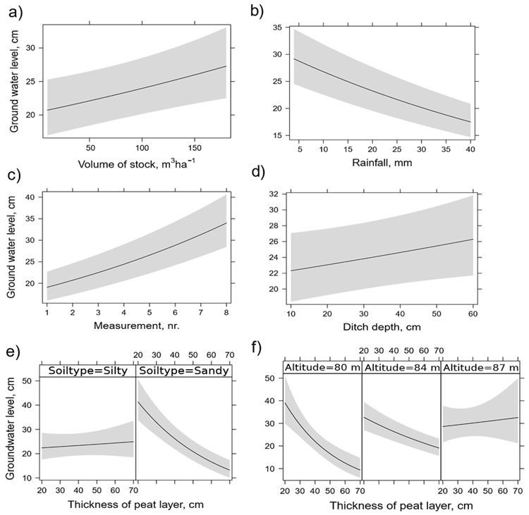
Fig. 3. The predictions of the continuous explanatory variables and their interactions for the ground water level model by predictors: volume of tree stock (a), rainfall (b), number of measurements during a growing season (c), ditch depth (d) and the interaction of soil type and ditch depth (e), altitude and thickness of peat layer (f). The predicted groundwater level values for the fifth (categorical) predictor variable peat type were: wooden-sphagnum type peat 21.7 cm and wooden-carex peat 25.3 cm. The other explanatory variables were fixed at their mean values (continuous variables) or at their average levels (for categorical variables, see Table 4).
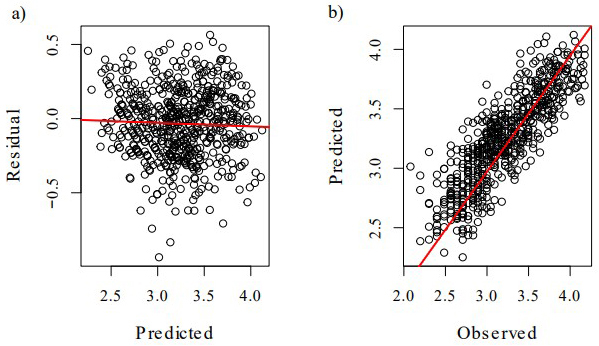
Fig. 4. Scatter plots for the predicted values vs. residuals (a) and observed vs. predicted values (b) of the model in the log-transformed scale. The values were computed using the fixed part of the model (marginal model).