Silva Fennica

Table 1. Average stand age (a [years]), average study plot area (A [ha]), stocking (N [trees ha^–1]), basal area at breast height (BA [m² ha^–1]), average diameter at breast height (DBH [cm]), mean height (H [m]), and growing stock (V [m³ ha^–1]) of the study sites.
	a	A	N	BA	DBH	H	V
Min	2	0.0002	2987	-	-	0.15	0.61
Max	14	0.0500	1555556	51.49	8.40	10.65	263.00
Mean	8	0.0135	144849	12.09	3.01	4.70	60.66
Median	7	0.0061	33194	10.50	1.55	3.23	35.53
Standard deviation	4	0.0148	345547	13.31	2.91	3.93	71.93

Table 2. Age (a [years]), diameter at ground level (d0 [cm]), diameter at breast height (dbh [cm]), height (h [m]), total aboveground (AB), stem (ST), branches (BR), and foliage (FL) dry biomass [kg] of the sampled trees.
Small trees
	a	d0		h	AB	ST	BR	FL
Min	1	0.23		0.26	0.0007	0.0004	0	0.0003
Max	5	1.30		1.27	0.0540	0.0286	0.0126	0.0143
Mean	3	0.77		0.71	0.0145	0.0066	0.0029	0.0050
Median	3	0.72		0.68	0.0095	0.0042	0.0019	0.0032
Standard deviation	1	0.26		0.28	0.0130	0.0066	0.0029	0.0042
Large trees
	a	d0	dbh	h	AB	ST	BR	FL
Min	3	0.90	0.10	1.41	0.0183	0.0128	0.0034	0.0021
Max	16	15.80	9.70	13.08	24.045	20.6267	4.2564	1.1328
Mean	9	5.78	3.22	5.57	3.5891	2.9820	0.4431	0.1740
Median	9	5.15	2.90	4.85	1.4377	1.0776	0.2414	0.1083
Standard deviation	4	3.41	2.17	2.96	5.4407	4.6867	0.6440	0.2114

Table 3. Goodness-of-fit measures (R² = coefficient of determination, RSE = residual standard error, BIC = Schwarz’s Bayesian information criterion, p-value = Shapiro-Wilk test result for residuals normality) for the best simplified (S) and expanded (E) models for estimating stem (ST), branches (BR), and foliage (FL) dry biomass in analyzed tree groups.
Model type and number			R²	RSE	BIC	p-value
Small trees (S for d0, E for d0 and h)
S	6	ST	0.6476	0.0040	–327.49	0.002
	6	BR	0.6528	0.0017	–396.07	0.018
	1	FL	0.7003	0.0023	–371.38	0.648
E	10	ST	0.9007	0.0021	–375.72	<0.0001
	13	BR	0.7165	0.0015	–408.09	0.087
	9	FL	0.7018	0.0023	–371.58	0.818
Large trees (S for dbh, E for dbh and h)
S	6	ST	0.9625	0.9110	405.40	<0.0001
	1	BR	0.8105	0.2813	57.56	<0.0001
	5	FL	0.7556	0.1052	–229.55	<0.0001
E	10	ST	0.9826	0.6226	296.69	<0.0001
	12	BR	0.8267	0.2700	49.36	<0.0001
	12	FL	0.7681	0.1025	–237.34	0.004
Large trees (S for d0, E for d0 and h)
S	6	ST	0.9270	1.2709	503.94	<0.0001
	1	BR	0.8196	0.2745	50.33	<0.0001
	5	FL	0.6865	0.1192	–192.71	<0.0001
E	10	ST	0.9733	0.7706	359.82	<0.0001
	12	BR	0.8196	0.2754	55.29	<0.0001
	12	FL	0.6866	0.1191	–192.76	<0.0001

Table 4. Parameters (a, b, c) with their standard errors (SE) and goodness-of-fit measures (R² = coefficient of determination, RSE = residual standard error, p-value = Shapiro-Wilk test result for residuals normality) for the final simplified (S) and expanded (E) models for small trees. All parameters are statistically significant at the significance level 0.05.
Model type and number			a	SE	b	SE	c	SE	R²	RSE	p-value
S	6+6+1	AB	-	-	-	-	-	-	0.7516	0.0068	0.3683
	6	ST	–1.91375	0.2144	–2.52269	0.2165	-	-	0.6653	0.0039	0.0506
	6	BR	–2.76320	0.2066	–2.51018	0.2085	-	-	0.6646	0.0017	0.0863
	1	FL	0.00807	0.0003	2.26422	0.1880	-	-	0.6982	0.0024	0.8324
E	10+13+9	AB	-	-	-	-	-	-	0.8768	0.0048	0.5060
	10	ST	0.01291	0.0004	1.28721	0.1880	1.875852	0.1935	0.9057	0.0021	0.0007
	13	BR	0.00537	0.0002	-	-	-	-	0.7286	0.0016	0.1216
	9	FL	0.00881	0.0004	0.77260	0.0619	-	-	0.7030	0.0024	0.9626

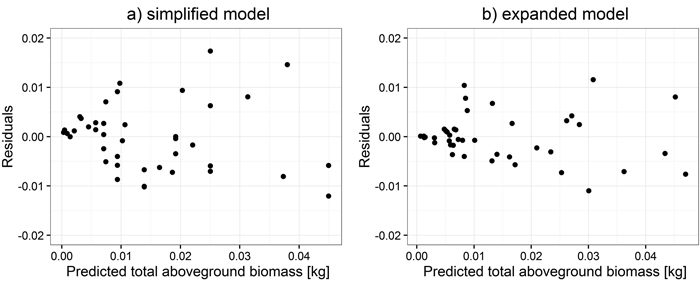
Fig. 1. Distribution of weighted residuals of simplified (a) and expanded (b) models for small trees.

Table 5. Parameters (a, b, c) with their standard errors (SE) and goodness-of-fit measures (R² = coefficient of determination, RSE = residual standard error, p-value = Shapiro-Wilk test result for residuals normality) for the final simplified (S) and expanded (E) models for large trees. All parameters are statistically significant at the significance level 0.05.
Model type and number			a	SE	b	SE	c	SE	R²	RSE	p-value
S	6+1+5	AB	-	-	-	-	-	-	0.9611	0.6997	<0.0001
	6	ST	4.55434	0.0556	–14.57160	0.3815	-	-	0.9616	0.5930	<0.0001
	1	BR	0.02126	0.0048	2.176631	0.1136	-	-	0.8235	0.1753	<0.0001
	5	FL	0.03489	0.0200	0.007996	0.0043	–2.09076	0.2573	0.7460	0.0713	<0.0001
E	10+12+12	AB	-	-	-	-	-	-	0.9752	0.5612	<0.0001
	10	ST	0.02606	0.0032	1.705293	0.0620	1.163906	0.0814	0.9820	0.4063	<0.0001
	12	BR	0.12882	0.0399	0.037619	0.0023	–0.04669	0.0126	0.8379	0.1683	<0.0001
	12	FL	0.06611	0.0180	0.011822	0.0010	–0.01331	0.00553	0.7561	0.0698	0.0046

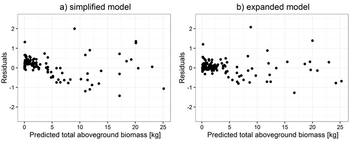
Fig. 2. Distribution of weighted residuals of simplified (a) and expanded (b) models for large trees.

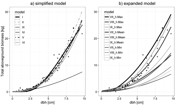
Fig. 3. Comparison to models from literature for large trees (black squares – measured total aboveground biomass). Simplified models (a): I – from this study (Table 4), II – Johansson (1999), III – Varik et al. (2009), IV and V Uri et al. (2012) models from Järvselja and Kambja respectively, VI – Liepiņš (2013). Expanded models (b): VII – form this study (Table 5), VIII – Repola (2008), IX – Smith et al. (2014) applied for minimum (h.Min), mean (h.Mean) and maximum (h.Max) height for all large trees.

Table 6. Goodness-of-fit measures (R² = coefficient of determination, RSE = residual standard error) for compared models (numbers defined in Fig. 3).
Model type and number	Simplified					Expanded
Model type and number	II	III	IV	V	VI	VIII	IX
R²	0.9395	0.9609	0.3249	0.9619	0.9474	0.9236	0.9698
RSE	1.3432	1.0799	4.4856	1.0656	1.2523	1.5141	0.9513

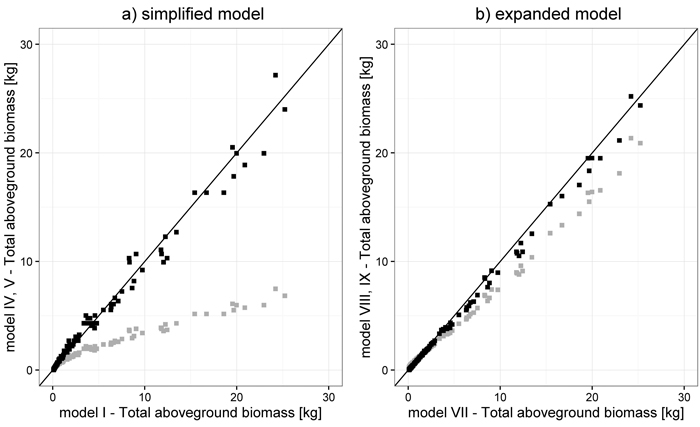
Fig. 4. Correlation between total aboveground biomass estimated with models developed in this study (model I and model VII) and estimated with the worst and best fitting models from the literature: model IV (grey) and model V (black), respectively, for simplified models (a) and model VIII (grey) and model IX (black), respectively, for expanded models (b) (model numbers are defined in Fig. 3).