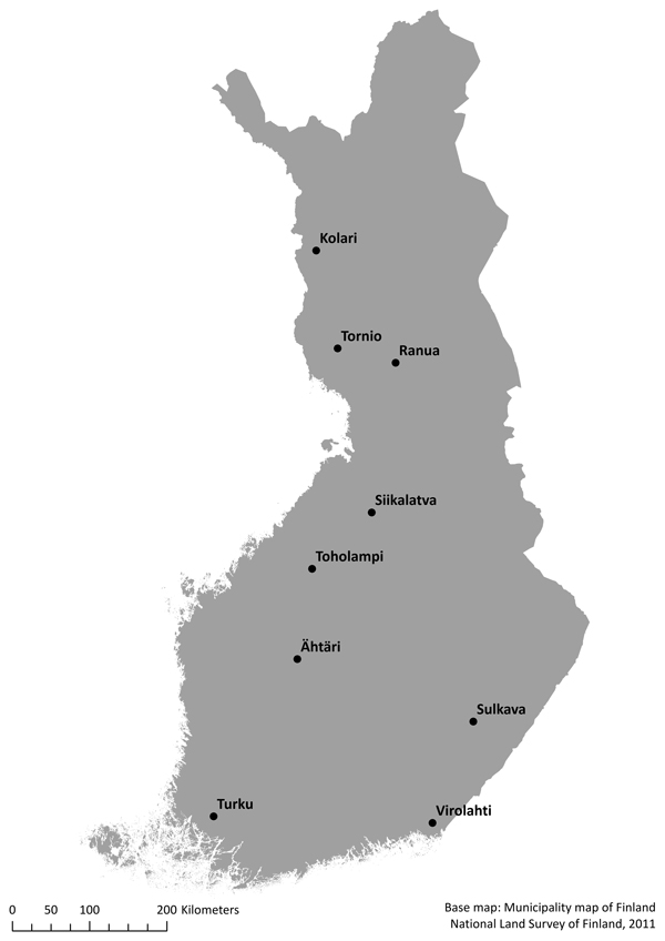
Fig. 1. Map of the inventory areas.
| Table 1. Field measurement dates, number of sample plots, observed mean volume, mean biomass and mean dominant height in each inventory area. Inventory areas are ordered from north to south. | |||||
| Inventory area | Time window | Number of sample plots | Volume (m3 ha–1) | Biomass (t ha–1) | Dominant height (m) |
| Kolari | 29.05.2013 – 07.10.2013 | 534 | 100.9 | 56.3 | 13.9 |
| Tornio | 28.05.2013 – 07.11.2013 | 596 | 97.2 | 57.3 | 12.7 |
| Ranua | 28.05.2012 – 24.10.2012 | 613 | 98.3 | 55.9 | 12.9 |
| Siikalatva | 20.06.2013 – 18.10.2013 | 657 | 118.0 | 64.4 | 15.6 |
| Toholampi | 26.07.2012 – 29.10.2012 | 587 | 102.8 | 55.8 | 14.7 |
| Ähtäri | 23.05.2013 – 25.10.2013 | 1233 | 139.7 | 73.9 | 16.8 |
| Sulkava | 01.07.2011 – 04.01.2012 | 570 | 173.4 | 90.3 | 18.6 |
| Virolahti | 13.05.2013 – 15.11.2013 | 724 | 179.4 | 93.5 | 17.8 |
| Turku | 23.04.2012 – 14.11.2012 | 716 | 180.9 | 93.6 | 18.8 |
| Table 2. Summary of distribution values for volume, biomass and dominant height by tree species for all of the sample plots in the modelling dataset. | ||||||
| Minimum | 1. Quartile | Median | Mean | 3. Quartile | Maximum | |
| Volume (m³ ha–1) | ||||||
| Pine | 0.0 | 8.3 | 54.2 | 71.8 | 110.5 | 572.4 |
| Spruce | 0.0 | 0.0 | 3.7 | 40.5 | 41.1 | 839.3 |
| Birch | 0.0 | 0.0 | 5.0 | 21.3 | 25.2 | 406.4 |
| Other d.t.* | 0.0 | 0.0 | 0.0 | 1.3 | 0.0 | 581.5 |
| Total | 3.0 | 63.1 | 114.1 | 134.9 | 184.3 | 915.5 |
| Biomass (t ha–1) | ||||||
| Pine | 0.0 | 4.7 | 28.8 | 36.7 | 57.3 | 244.4 |
| Spruce | 0.0 | 0.0 | 2.7 | 22.8 | 26.4 | 366.1 |
| Birch | 0.0 | 0.0 | 2.8 | 12.2 | 14.6 | 206.6 |
| Other d.t.* | 0.0 | 0.0 | 0.0 | 0.7 | 0.0 | 302.5 |
| Total | 1.8 | 36.0 | 62.9 | 72.4 | 98.6 | 409.1 |
| Dominant height (m) | ||||||
| Total | 3.9 | 12.1 | 15.9 | 16.0 | 19.5 | 32.9 |
| * Other deciduous trees | ||||||
| Table 3. The sensor models, sensor units (A–D), scanning time windows, flying altitudes, pulse repetition frequencies (PRF), half scan angles, and mean pulse density for each project. | |||||||
| Inventory area | Sensor model | Sensor unit | Time window | Altitude (m) | PRF (hz) | Half scan angle (degrees) | Pulse density (pl/m2) |
| Kolari | Optech ALTM Gemini | B | 07.06. – 06.08.2013 | 1950 | 50 000 | 15 | 0.6 |
| Tornio | Leica ALS 70-HA | C | 13.06. – 04.08.2013 | 1950 | 71 000 | 20 | 0.5 |
| Ranua | Optech ALTM Gemini | A | 04.07. – 24.08.2012 | 1750 | 70 000 | 20 | 1.0 |
| Siikalatva | Optech ALTM Gemini | B | 12.06. – 20.06.2013 | 1950 | 50 000 | 15 | 0.9 |
| Toholampi | Optech ALTM Gemini | B | 28.06. – 03.07.2012 | 1750 | 70 000 | 20 | 1.0 |
| Ähtäri | Optech ALTM Gemini | A | 28.06. – 27.08.2013 | 1730 | 70 000 | 20 | 0.7 |
| Sulkava | Optech ALTM Gemini | A | 31.07. – 04.09.2011 | 2000 | 50 000 | 15 | 0.7 |
| Virolahti | Leica ALS 70-HA | D | 25.06. – 03.07.2013 | 1900 | 71 800 | 20 | 0.7 |
| Turku | Optech ALTM Gemini | B | 13.06. – 22.06.2012 | 1750 | 70 000 | 20 | 1.0 |
| Table 4. Root mean square error (RMSE), mean difference (MD) and t-test statistics of the region-specific nationwide volume model predictions. | ||||
| Inventory Area | RMSE-% | MD-% | t-value | p-value |
| Kolari | 30.1 | 15.4 | 13.7 | < 2.2×10⁻¹⁶ |
| Tornio | 28.4 | –7.4 | –6.6 | 8.5×10⁻¹¹ |
| Ranua | 31.8 | 16.3 | 14.7 | < 2.2×10⁻¹⁶ |
| Siikalatva | 25.8 | –3.6 | –3.6 | 2.9×10⁻⁴ |
| Toholampi | 24.8 | –5.5 | –5.5 | 5.4×10⁻⁸ |
| Ähtäri | 26.8 | 8.0 | 11.1 | < 2.2×10⁻¹⁶ |
| Sulkava | 30.4 | –11.2 | –9.5 | < 2.2×10⁻¹⁶ |
| Virolahti | 26.8 | –6.4 | –6.6 | 9.0×10⁻¹¹ |
| Turku | 22.9 | –1.7 | –2.0 | 5.1×10⁻² |
| Table 5. Regional volume (V) models, their residual variances (σ2) and relative root mean square error (RMSE) values. The used ALS metrics (Section 2.4) were means (havgF and havgL), standard deviations (hstdF and hstdL), height quantiles (h70F, h90F, h95L and h99L) and density percentages (veg3F, veg9L and veg19L) of first (F) and last (L) echoes, and the maximum value of last echoes (hmaxL). | ||||
| Inventory area | σ² | RMSE-% | ||
| Kolari | (18) | 0.9607 | 21.5 | |
| Tornio | (19) | - | 24.0 | |
| Ranua | (20) | 1.1578 | 22.9 | |
| Siikalatva | (21) | 1.4291 | 24.4 | |
| Toholampi | (22) | 1.1254 | 24.0 | |
| Ähtäri | (23) | 1.5484 | 24.7 | |
| Sulkava | (24) | 3.2302 | 26.6 | |
| Virolahti | (25) | 2.3953 | 24.8 | |
| Turku | (26) | 1.8838 | 21.8 | |

Fig. 2. Predicted (m3 ha–1) values of nationwide and regional volume models plotted against observed values (m3 ha–1) in the modeling dataset. View larger in new window/tab.
| Table 6. Root mean square error (RMSE), mean difference (MD) and t-test statistics of the region-specific nationwide biomass model predictions. | ||||
| Inventory Area | RMSE-% | MD-% | t-value | p-value |
| Kolari | 29.7 | 11.1 | 9.3 | < 2.2×10⁻¹⁶ |
| Tornio | 29.4 | –2.9 | –2.4 | 1.7×10⁻² |
| Ranua | 32.6 | 16.5 | 14.6 | < 2.2×10⁻¹⁶ |
| Siikalatva | 25.9 | –7.1 | –7.3 | 8.9×10⁻¹³ |
| Toholampi | 25.3 | –6.8 | –6.8 | 2.8×10⁻¹¹ |
| Ähtäri | 26.0 | 8.2 | 11.6 | < 2.2×10⁻¹⁶ |
| Sulkava | 29.4 | –11.9 | –10.6 | < 2.2×10⁻¹⁶ |
| Virolahti | 26.0 | –3.9 | –4.0 | 5.9×10⁻⁵ |
| Turku | 22.2 | –2.3 | –2.7 | 6.4×10⁻³ |
| Table 7. Regional biomass (Mt) models, their residual variances (σ2) and relative root mean square error (RMSE) values. The used ALS metrics (Section 2.4) were means (havgF, and havgL), height quantiles (h70F, h90F and h99L) and density percentages (veg3F, veg7L, veg8L and veg19L) of first (F) and last (L) echoes, standard deviation (hstdL), and the maximum value (hmaxL) of last echoes. | ||||
| Inventory area | σ² | RMSE-% | ||
| Kolari | (28) | 0.5603 | 22.0 | |
| Tornio | (29) | 0.6791 | 23.7 | |
| Ranua | (30) | 0.6465 | 23.4 | |
| Siikalatva | (31) | 0.7214 | 23.0 | |
| Toholampi | (32) | 0.5734 | 23.0 | |
| Ähtäri | (33) | 0.8074 | 23.4 | |
| Sulkava | (34) | 1.6063 | 25.2 | |
| Virolahti | (35) | 1.2081 | 23.4 | |
| Turku | (36) | 0.8717 | 20.1 | |
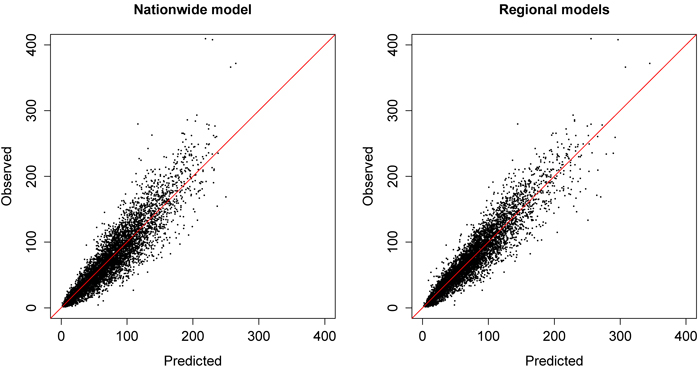
Fig. 3. Predicted (t ha–1) values of nationwide and regional biomass models plotted against observed values (t ha–1) in the modelling dataset. View larger in new window/tab.
| Table 8. Root mean square error (RMSE), mean difference (MD) and t-test statistics of the region-specific nationwide dominant height model predictions. | ||||
| Inventory Area | RMSE-% | MD-% | t-value | p-value |
| Kolari | 7.2 | –0.4 | –1.2 | 2.2×10⁻¹ |
| Tornio | 10.5 | –8.0 | –28.8 | < 2.2×10⁻¹⁶ |
| Ranua | 7.6 | –1.7 | –5.7 | 2.3×10⁻⁸ |
| Siikalatva | 5.5 | 1.6 | 7.6 | 1.2×10⁻¹³ |
| Toholampi | 5.9 | 0.7 | 3.0 | 2.8×10⁻³ |
| Ähtäri | 6.5 | 1.4 | 7.5 | 1.4×10⁻¹³ |
| Sulkava | 6.9 | –0.8 | –2.7 | 7.7×10⁻³ |
| Virolahti | 5.4 | 0.2 | 1.1 | 2.9×10⁻¹ |
| Turku | 5.9 | 2.4 | 11.8 | < 2.2×10⁻¹⁶ |
| Table 9. Regional dominant height (HDOM) models, their residual variances (σ2) and relative root mean square error (RMSE) values. The used ALS metrics (Section 2.4) were height quantiles (h95F, h99F, h95L and h99L) of first (F) and last (L) echoes. | ||||
| Inventory Area | σ² | RMSE-% | ||
| Kolari | (38) | 0.0161 | 6.5 | |
| Tornio | (39) | - | 6.4 | |
| Ranua | (40) | - | 6.3 | |
| Siikalatva | (41) | - | 5.2 | |
| Toholampi | (42) | 0.0127 | 5.8 | |
| Ähtäri | (43) | - | 6.3 | |
| Sulkava | (44) | 0.0248 | 6.7 | |
| Virolahti | (45) | - | 5.4 | |
| Turku | (46) | - | 5.4 | |
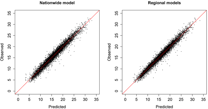
Fig. 4. Predicted (m) values of nationwide dominant height model and regional models plotted against observed values (m) in the modeling dataset. View larger in new window/tab.
| Table 10. Relative root mean square error (RMSE) and mean difference (MD) values of cross-validated nationwide (leave-inventory-area-out) and regional (leave-plot-out) volume, biomass and dominant height models, and the calibrated nationwide models in different inventory areas. | ||||||
| RMSE-% | MD-% | |||||
| Inventory area | Nationwide | Calibrated | Regional | Nationwide | Calibrated | |
| Volume | Kolari | 31.0 | 23.9 | 21.7 | 16.8 | 3.9 |
| Tornio | 28.9 | 27.5 | 24.2 | –8.8 | –1.5 | |
| Ranua | 32.9 | 26.3 | 23.1 | 18.2 | 3.5 | |
| Siikalatva | 25.9 | 26.4 | 24.6 | –4.2 | –2.3 | |
| Toholampi | 25.0 | 24.7 | 24.3 | –6.1 | –1.9 | |
| Ähtäri | 28.0 | 26.0 | 24.8 | 10.8 | 0.8 | |
| Sulkava | 31.6 | 28.3 | 26.8 | –13.2 | –1.2 | |
| Virolahti | 27.0 | 26.7 | 25.0 | –7.5 | –0.6 | |
| Turku | 23.0 | 23.3 | 21.9 | –2.0 | –0.3 | |
| Biomass | Kolari | 30.1 | 26.3 | 22.2 | 12.1 | 2.9 |
| Tornio | 29.6 | 29.0 | 23.9 | –3.5 | –0.3 | |
| Ranua | 33.8 | 27.7 | 23.6 | 18.7 | 4.3 | |
| Siikalatva | 26.1 | 25.5 | 23.2 | –8.0 | –2.8 | |
| Toholampi | 25.6 | 24.4 | 23.2 | –7.6 | –1.9 | |
| Ähtäri | 27.3 | 24.1 | 23.5 | 10.8 | 1.5 | |
| Sulkava | 30.3 | 27.0 | 25.4 | –13.8 | –1.7 | |
| Virolahti | 26.1 | 25.7 | 23.6 | –4.4 | –0.1 | |
| Turku | 22.3 | 21.9 | 20.2 | –2.6 | –0.3 | |
| Dominant height | Kolari | 7.2 | 7.4 | 6.5 | –0.4 | 0.0 |
| Tornio | 11.4 | 8.2 | 6.4 | –9.1 | –4.6 | |
| Ranua | 7.7 | 7.6 | 6.3 | –2.0 | –0.3 | |
| Siikalatva | 5.5 | 5.3 | 5.2 | 1.7 | 0.4 | |
| Toholampi | 6.0 | 5.9 | 5.8 | 0.8 | 0.1 | |
| Ähtäri | 6.6 | 6.4 | 6.3 | 1.7 | 0.3 | |
| Sulkava | 6.9 | 6.9 | 6.7 | –0.9 | –0.2 | |
| Virolahti | 5.4 | 5.5 | 5.4 | 0.2 | 0.1 | |
| Turku | 6.1 | 5.6 | 5.4 | 2.8 | 0.9 | |
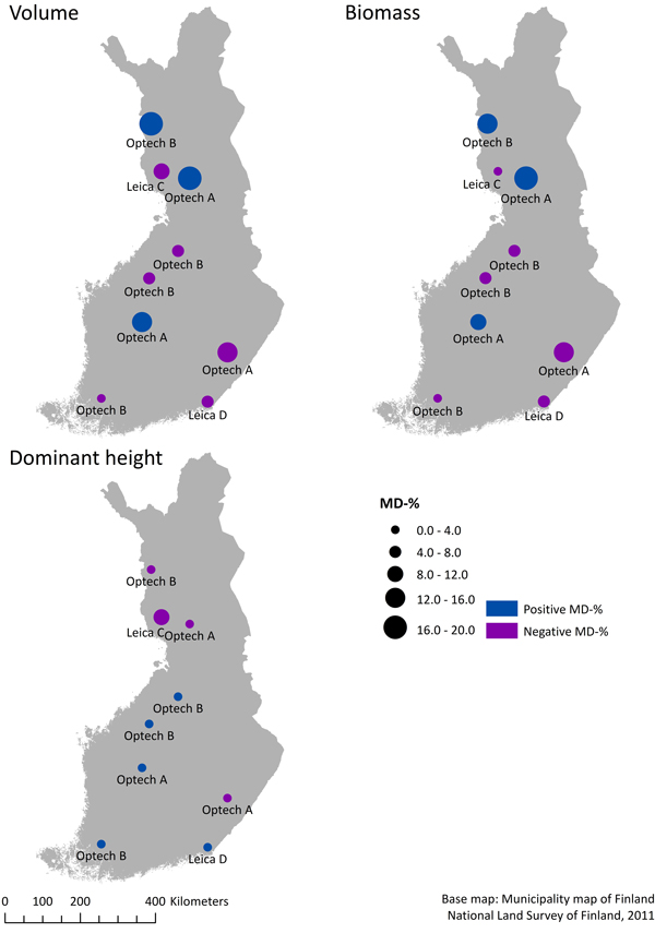
Fig. 5. Map of the mean difference (MD) values of nationwide volume, biomass and dominant height models with information of different sensor models (Optech/Leica) and sensor units (A–D).
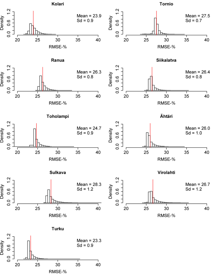
Fig. 6. Root mean square error (RMSE) distributions of the 10 000 times calibrated nationwide volume model in each inventory area. The red line represents the mean of the distribution. Sd = Standard deviation. View larger in new window/tab.
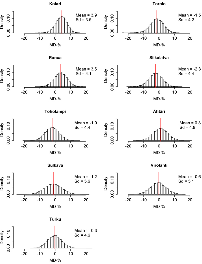
Fig. 7. Mean difference (MD) distributions of the 10 000 times calibrated nationwide volume model in each inventory area. The red line represents the mean of the distribution. Sd = Standard deviation. View larger in new window/tab
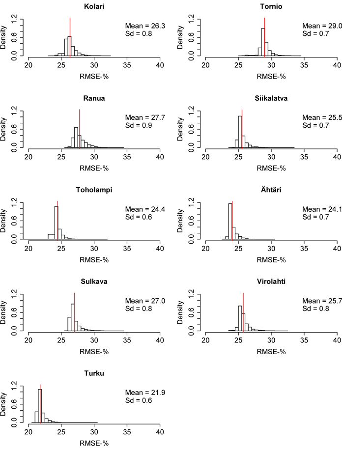
Fig. 8. Root mean square error (RMSE) distributions of the 10 000 times calibrated nationwide biomass model in each inventory area. The red line represents the mean of the distribution. Sd = Standard deviation. View larger in new window/tab
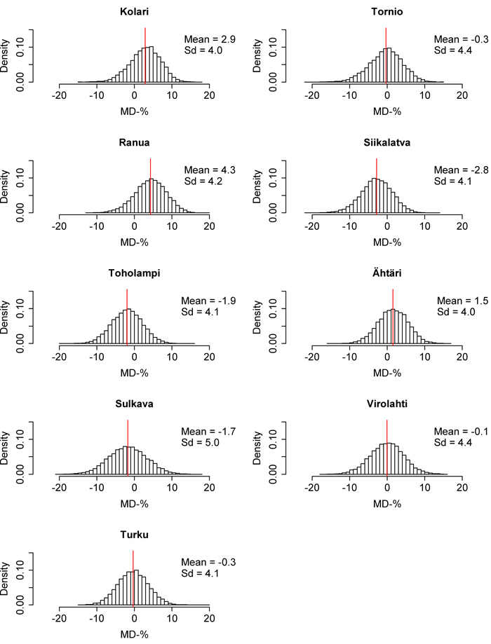
Fig. 9. Mean difference (MD) distributions of the 10 000 times calibrated nationwide biomass model in each inventory area. The red line represents the mean of the distribution. Sd = Standard deviation. View larger in new window/tab
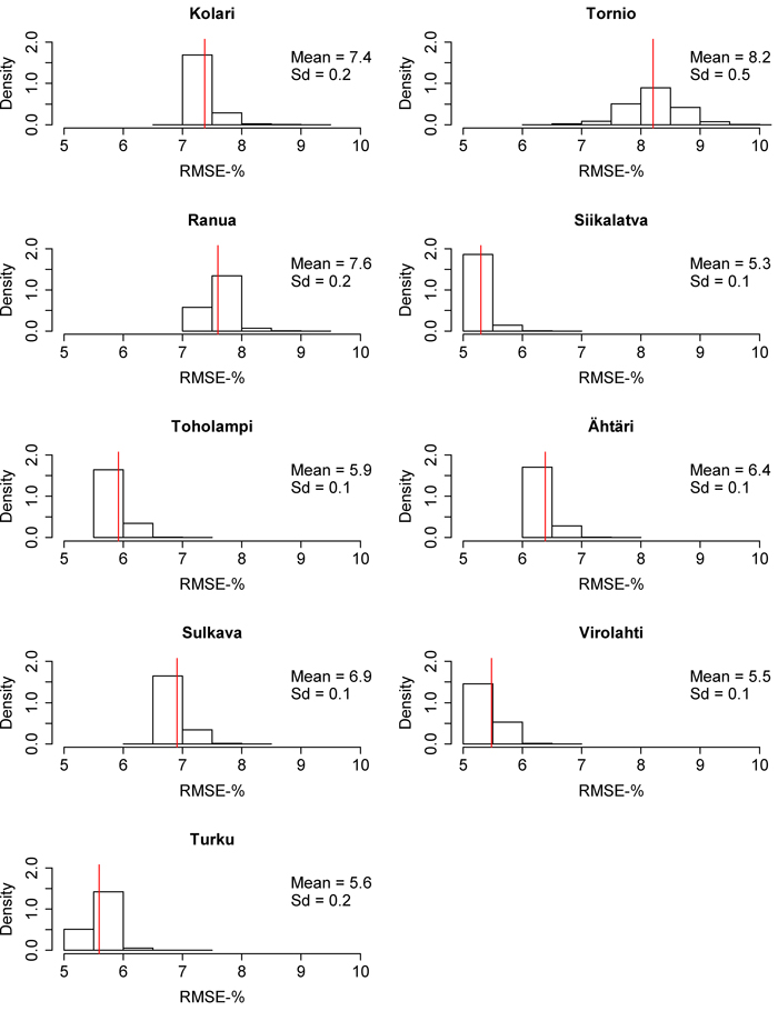
Fig. 10. Root mean square error (RMSE) distributions of the 10 000 times calibrated nationwide dominant height model in each inventory area. The red line represents the mean of the distribution. Sd = Standard deviation. View larger in new window/tab
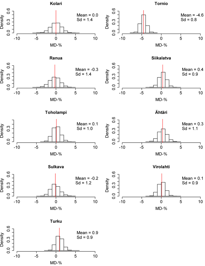
Fig. 11. Mean difference (MD) distributions of the 10 000 times calibrated nationwide dominant height model in each inventory area. The red line represents the mean of the distribution. Sd = Standard deviation. View larger in new window/tab