| Table 1. Compartment information. | |
| Harvesting contractor | Mecharv |
| Grower company | CMPC – Forestal Mininco |
| Farm | Totoras |
| Compartment number | 3 |
| Species | Eucalyptus globulus Labill. |
| Established (year/month) | 1998/05 |
| Treatment | Clear-cut |
| Fell age (years/months) | 9/11 |
| Average tree volume (m3) | 0.204 |
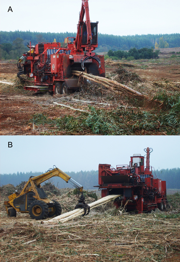
Fig. 1. The chain flail delimber debarker at work: A) feeding whole trees and B) discharging debarked stems.
| Table 2. Volume, bark-wood bond strength (BWBS) and work quality classes. | |
| Volume class | Volume range (m3 ub) |
| 1. Very small | < 0.050 |
| 2. Small | 0.051–0.099 |
| 3. Medium | 0.100–0.199 |
| 4. Large | 0.200–0.299 |
| 5. Very large | 0.300–0.499 |
| BWBS class | Description |
| 1. Very good | The bark comes off in a very long strip that can reach into the canopy before it severs (>10 m) |
| 2. Good | The bark comes off in long strips of half of the height of the tree (approximately from 4 to 10 m) |
| 3. Medium | The bark comes off in medium lengths of between one and four metres |
| 4. Poor | The bark comes off in short lengths of up to one metre |
| 5. Very poor | The bark will not come off by hand; it needs to be chiselled off by means of the hatchet |
| Quality class | Description |
| 1. Good | All bark is removed from the stem: residual bark content estimated to less than 0.5 % achieved |
| 2. Medium | Strips of residual bark remain: residual bark content estimated to less than 1 % achieved |
| 3. Poor | Sections of the tree have not had bark removed: residual bark content estimated to more than 1 % |
| Table 3. Main results of the productivity study. | |||||
| mean | SD | min | max | ||
| Cycle time | s | 42 | 11 | 14 | 116 |
| Trees in load | n° | 4.4 | 1.6 | 1 | 11 |
| Load volume | m3 ub | 0.857 | 0.338 | 0.025 | 2.050 |
| Tree volume | m3 ub | 0.204 | 0.078 | 0.025 | 0.475 |
| Productivity | m3 ub PMH–1 | 74.7 | 28.6 | 3.2 | 201.5 |
| m3 ub SMH–1 | 59.1 | 22.6 | 2.5 | 159.4 | |
| Utilization | % | 80.5 | - | - | - |
| DF | 0.24 | - | - | - | |
| SD = standard deviation; ub = under bark; PMH = productive machine hours, excluding delays; SMH = scheduled machine hours, including delays; Utilization = productive time/scheduled time; DF = delay factor, or delay time/productive time, where productive time is expressed in PMH | |||||
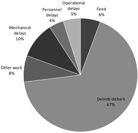
Fig. 2. Breakdown of work site time by productive tasks and delays. Other work = handling loads and residues, re-arranging stacks.
| Table 4. Results of the regression analysis. | ||||
| Productive time per cycle (s) = a + b × Load volume (m3 ub) | ||||
| n = 788 | R2 adjusted = 0.220 | |||
| Anova Table | ||||
| DF | SS | F-value | P-Value | |
| Regression | 1 | 372.00 | 222.41 | <0.0001 |
| Residual | 786 | 1314.72 | - | - |
| Total | 787 | 1686.72 | - | - |
| Regression Coefficients | ||||
| Coeff | SE | F-value | P-Value | |
| a | 28.50 | 0.96 | 29.30 | <0.0001 |
| b | 15.78 | 1.08 | 14.19 | <0.0001 |
| Load volume (m3 ub) = a + b ln Tree volume (m3 ub) | ||||
| n = 788 | R2 adjusted = 0.327 | |||
| Anova Table | ||||
| DF | SS | F-value | P-Value | |
| Regression | 1 | 29.43 | 383.56 | <0.0001 |
| Residual | 786 | 60.30 | - | - |
| Total | 787 | 89.73 | - | - |
| Regression Coefficients | ||||
| Coeff | SE | F-value | P-Value | |
| a | 1.63 | 0.04 | 39.97 | <0.0001 |
| b | 0.47 | 0.02 | 19.58 | <0.0001 |
| DF = degrees of freedom; SS = sum of squares; Coeff = coefficient; SE = standard error | ||||
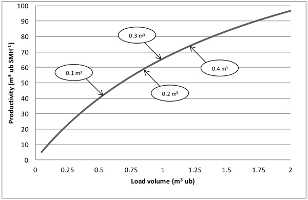
Fig. 3. Relationship between productivity and load volume. SMH = scheduled machine hours, including delays; the arrows indicate the position on the graph corresponding to the mean tree volume (m3 ub) indicated in the ellipses, based on the second equation shown in Table 4.
| Table 5. Product quality vs. BWBS class. | ||||||
| BWBS 3 | BWBS 4 | BWBS 5 | Total | % | ||
| Quality 1 | n | 369 | 150 | 122 | 641 | 57.9 |
| % | 57.6 | 23.4 | 19.0 | 100.0 | ||
| Quality 2 | n | 56 | 49 | 214 | 319 | 28.8 |
| % | 17.6 | 15.4 | 67.1 | 100.0 | ||
| Quality 3 | n | 10 | 6 | 132 | 148 | 13.4 |
| % | 6.8 | 4.1 | 89.2 | 100.0 | ||
| Total | n | 435 | 205 | 468 | 1108 | |
| % | 39.3 | 18.5 | 42.2 | 100.0 | ||
| χ2 = 365.12, P-Value < 0.0001 | ||||||
| BWBS = bark-wood bond strength | ||||||
| Table 6. Results of the ordinal logistic regression analysis. | |||||
| n = 1108 | |||||
| R2 = 0.232 | |||||
| Quality class 2 | |||||
| Coeff | SE | e Coeff | χ2 | P-Value | |
| Constant | –3.998 | 0.310 | 0.018 | 166.257 | <0.0001 |
| BWBS 4 | 0.821 | 0.224 | 2.272 | 13.378 | 0.0003 |
| BWBS 5 | 2.158 | 0.190 | 8.656 | 128.792 | <0.0001 |
| n° trees | 0.485 | 0.060 | 1.624 | 65.835 | <0.0001 |
| Quality class 3 | |||||
| Coeff | SE | e Coeff | χ2 | P-Value | |
| Constant | –6.062 | 0.465 | 0.002 | 169.744 | <0.0001 |
| BWBS 4 | 0.455 | 0.529 | 1.576 | 0.740 | 0.3896 |
| BWBS 5 | 3.326 | 0.350 | 27.833 | 90.128 | <0.0001 |
| n° trees | 0.556 | 0.071 | 1.744 | 61.518 | <0.0001 |
| BWBS = bark-wood bond strength; Coeff = coefficient; SE = standard error; n° trees = number of trees in a load | |||||
| Table 7. Results of previous chain flail studies. View in new window/tab. |