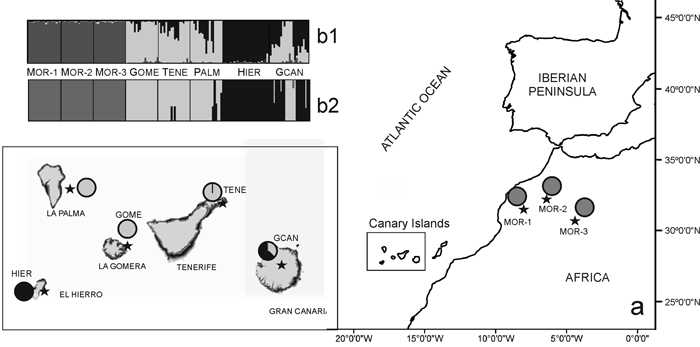
Fig. 1. (a) Location map and Bayesian analysis of the genetic structure of 175 individuals from eight sampled populations of Juniperus turbinata. The great rectangle that includes Canary Islands represent an enlargement of the same area in the small rectangle Pie charts represent the mean proportion of membership of each population to the predefined K = 3 clusters with BAPS. (b) Plots show the membership of individuals to the predefined K = 3 clusters obtanined with b1, STRUCTURE and b2, BAPS. Number and codes of populations are listed in Table 1. View larger in new window/tab.
| Table 1. Geographical location of eight sampled populations of Juniperus turbinata and genetic diversity estimates. N = Number of individuals sampled per population; PLP = Percentage of polymorphic loci; He = Expected heterozygosity (Nei’s gene diversity); Hs = Mean Nei’s gene diversity within populations; Ht = Total gene diversity; Fst = Index of population differentiation. | ||||||||
| Pop | Island/*Country | Location | N | PLP | He | Hs | Ht | Fst |
| MOR-1 | Morocco* | 31°35´N, 07°76´W | 20 | 67.7 | 0.217 | |||
| MOR-2 | Morocco* | 32°18´N, 06°53´W | 20 | 65.0 | 0.207 | |||
| MOR-3 | Morocco* | 32°61´N, 04°53´W | 20 | 66.2 | 0.203 | |||
| GOME | La Gomera | 28°19´N, 17°26´W | 20 | 69.6 | 0.214 | |||
| TENE | Tenerife | 28°56´N, 16°24´W | 20 | 68.3 | 0.213 | |||
| PALM | La Palma | 28°68´N, 17°77´W | 20 | 73.7 | 0.218 | |||
| HIER | El Hierro | 27°75´N, 18°13´W | 30 | 68.4 | 0.192 | |||
| GCAN | Gran Canaria | 28°01´N, 15°65´W | 25 | 67.4 | 0.211 | |||
| TOTAL | 175 | 94.1 | 0.209 | 0.243 | 0.1398 | |||
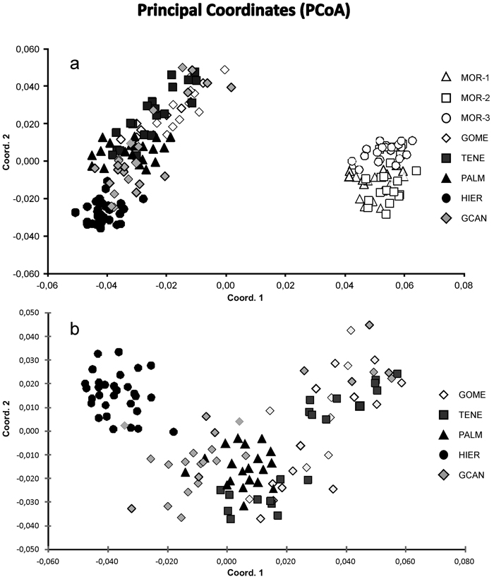
Fig. 2. Principal coordinate analysis of the 175 individuals from eight sampled populations of J. turbinata based on pair-wise Nei’s (1978) genetic distances. (a) Scatter plot showing eight populations based on two first components of the PCoA. (b) Scatter plot showing 115 individuals from five Canarian populations. Number and codes of populations are listed in Table 1.
| Table 2. Pairwise estimate Fst values among eight populations of J. turbinata. All values are significant at 0.001 level. Number and codes of populations are listed in Table 1. | ||||||||
| MOR-1 | MOR-2 | MOR-3 | GOME | TENE | PALM | HIER | GCAN | |
| MOR-1 | 0.000 | |||||||
| MOR-2 | 0.042 | 0.000 | ||||||
| MOR-3 | 0.067 | 0.051 | 0.000 | |||||
| GOME | 0.152 | 0.159 | 0.155 | 0.000 | ||||
| TENE | 0.185 | 0.192 | 0.197 | 0.016 | 0.000 | |||
| PALM | 0.193 | 0.206 | 0.212 | 0.037 | 0.046 | 0.000 | ||
| HIER | 0.254 | 0.265 | 0.276 | 0.120 | 0.114 | 0.071 | 0.000 | |
| GCAN | 0.181 | 0.190 | 0.188 | 0.033 | 0.039 | 0.021 | 0.068 | 0.000 |
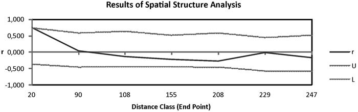
Fig. 3. Correlogram from spatial autocorrelation analysis using the correlation coefficient r, and variable distance classes. 95% confidence error bars for r were estimated by bootstrapping over pairs of samples; dashed lines (U, L) represent upper and lower bounds of a 95% CI for r generated under the null hypothesis of random geographic distribution.