Silva Fennica

Table 1. The geographical characteristics of four populations of C. sativa in Hyrcanian forest and the sample size in each population.
Population name	Latitude, Longitude	Altitude (m a.s.l.)	Sample size (No.)	Population size (Hectare)
Veysroud (V)	37°16´N, 49°15´E	211–711	8	60
Shafaroud (SH)	37°30´N, 49°02´E	200–360	8	50
Siyahmazgi (S)	40°97´N, 35°49´E	290–350	8	40
QaleRoudkhan (R)	37°05´N, 49°14´E	200–400	8	50

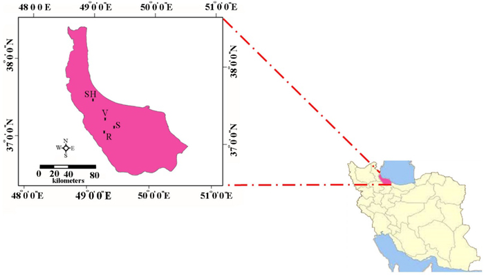
Fig. 1. The geographical positions of Hyrcanian populations of C. sativa in North of Iran. R = QalehRoudkhan region; S = SiyahMazgi region; SH = Shafaroud region; V = Veysroud region.

Table 2. Sequences of Castanea SSR primer pairs, PCR annealing temperature and PCR expected product size.
Marker	Number	SSR locus		Primer sequences (5’ → 3’)	Ta (°C)	Size of alleles (bp)	Reference
NU SSR	1	CsCAT 1	F	GAGAATGCCCACTTTTGCA	54	177–212	Marinoni et al. 2003
			R	GCTCCCTTATGGTCTCG
	2	CsCAT 3	F	CACTATTTTATCATGGACGG	58	179–198
			R	CGAATTGAGAGTTCATACTC
	3	CsCAT 6	F	AGTGCTCGTGGTCAGTGAG	54	199–238
			R	CAACTCTGCATGATAAC
	4	CsCAT 7	F	GAACATGATGATTGGCCTC	54	179–223
			R	CCAAACATGACATATGTCCC
	5	CsCAT 14	F	CGAGGTTGTTGTTCATCATTAC	54	133–151
			R	GATCTCAAGTCAAAAGGTGTC
	6	CsCAT 15	F	TTCTGCGACCTCGAAACCGA	56	123–155
			R	GCTAGGGTTTTCATTTCTAG
	7	CsCAT 17	F	TTGGCTATACTTGTTCTGCAAG	56	132–151
			R	GCCCCATGTTTTCTTCCATGG
	8	CsCAT 41	F	AAGTCAGCAACACCATATGC	58	199–238
			R	CCCACTGTTCATGAGTTTCT
	9	EMC 38	F	TTTCCCTATTTCTAGTTTGTGATG	58	227–261	Buck et al. 2003
			R	ATGGCGCTTTGGATGAAC
	10	QpZAG110	F	GGAGGCTTCCTTCAACCTACT	54	207–223	Steinkellner et al. 1997
			R	GATCTCTTGTGTGCTGTATTT
CP SSR	1	CCMP2	F	GATCCCGGACGTAATCCTG	55	234	Weising and Gardner 1999
			R	ATCGTACCGAGGGTTCGAAT
	2	CCMP4	F	AATGCTGAATCGAYGACCTA	55	114
			R	CCAAAATATTBGGAGGACTCT
	3	CCMP10	F	TTTTTTTTTAGTGAACGTGTCA	55	113
			R	TTCGTCGDCGTAGTAAATAG
	4	CMCS2	F	GAGCCATTCCCTTTTAGAAT	55	141	Sebastiani et al. 2004
			R	TTGAAAACCGGTATAGTTCG
	5	CMCS7	F	AAGCGAGATGAATGAGTTTT	55	205
			R	AAAATTGGATTGATTATTGACT
	6	CMCS8	F	GGTCTATTTTTCCACTCACAA	55	179
			R	AGAAATAAACACCCCCATTA
	7	CMCS12	F	ATATTGGTAAAACGGCAACT	55	216
			R	TTTATGGCATGAAACAACTC
	8	CMCS14	F	GGATTGTAACAAATTTTTCAGG	55	176
			R	GTGCAAGGAATGTCGAACTA
F = forward primer; R = reverse primer; SSR = Simple sequence repeat; CP SSR = Chloroplast SSR; NU SSR = Nuclear SSR; Ta = PCR annealing temperature

Table 3. Genetic variability within four C. sativa populations based on SSR markers.
Marker	Pop		N	Na	Ne	I	H_o	H_e	UH_e	F
NU SSR	R	Mean	8.000	3.000	2.142	0.807	0.538	0.463	0.494	–0.147
	R	SE	0.000	0.365	0.243	0.133	0.110	0.074	0.078	0.125
	S	Mean	8.000	2.400	1.903	0.679	0.563	0.434	0.463	–0.293
	S	SE	0.000	0.221	0.148	0.093	0.112	0.059	0.063	0.166
	SH	Mean	8.000	3.300	2.435	0.962	0.675	0.559	0.597	–0.230
	SH	SE	0.000	0.213	0.197	0.081	0.075	0.044	0.046	0.130
	V	Mean	8.000	2.700	2.174	0.781	0.475	0.477	0.508	–0.007
	V	SE	0.000	0.260	0.223	0.122	0.096	0.073	0.078	0.115
	Total	Mean	8.000	2.85	2.163	0.630	0.563	0.512	0.516	–0.169
	Total	SE	0.000	0.265	0.203	0.107	0.098	0.063	0.071	0.134
NU SSR = Nuclear SSR; R = QalehRoudkhan region; S = SiyahMazgi region; SH = Shafaroud region; V = Veysroud region; N = number of individuals analyzed; Na = number of alleles; Ne = effective number of alleles; I = Shannon index; H_o = observed heterozygosity; H_e = expected heterozygosity; UH_e = unbiased expected heterozygosity; F = F-values; SE = Standard errors

Table 4. Analyses of molecular variance (AMOVA) for four populations of C. sativa from Hyrcanian forest by Nuclear SSR (NU SSR). Statistics include sums of squared deviations (SS); mean squared deviations (MS), variance component estimates (Est. Var.), the percentage of the total variance contributed by each component; estimator of relative genetic differentiation based on fraction of total variance of allele size between two subpopulations (R_st) and the probability of obtaining a more extreme component estimate by chance alone.
Marker	S.O.V.	D.f	SS	MS	Est. Var.	% of Variance
NU SSR	Between groups	3	8.305.094	2.768.365	130.923	16%
	Within groups	60	40.415.375	673.590	673.590	84%
	Total Sum	63	48.720.469		804.513	100%

	Stat	Value(Φ)	P(rand > = data)
	R_st	0.163	0.010

Table 5. Pairwise estimated of Nei’s genetic distance and the calculated Fst based on 10 nuclear SSR markers among four populations of C. sativa in Hyrcanian forest.
	Population	R	S	SH
Nei distance	R	0.000
	S	0.215
	SH	0.237	0.175	0.000
	V	0.012	0.095	0.208
F_st	R	0.000
	S	0.132	0.000
	SH	0.185	0.148	0.000
	V	0.034	0.114	0.163
NU SSR = Nuclear SSR; R = QalehRoudkhan region; S = SiyahMazgi region; SH = Shafaroud region; V = Veysroud region; F_st = Fixation index

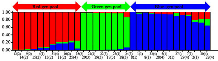
Fig. 2. Population structure of C. sativa was estimated based on Structure analysis. In the figure, the individuals of Iranian Castanea were sorted by Bayesian clustering approaches based on 10 nuclear microsatellite loci. Each bar represents a single individual analyzed. Legend of number in brackets: 1 = R1; 2 = R2; 3 = R3; 4 = R4; 5 = R5; 6 = R6; 7 = R7; 8 = R8; 9 = S1; 10 = S2; 11 = S3; 12 = S4; 13 = S5; 14 = S6; 15 = S7; 16 = S8; 17 = SH1; 18 = SH2; 19 = SH3; 20 = SH4; 21 = SH5; 22 = SH7; 23 = SH10; 24 = SH12; 25 = V1; 26 = V2; 27 = V3; 28 = V4; 29 = V5; 30 = V6; 31 = V7; 32 = V8.

Table 6. The proportion membership of each individual of the four populations in each of the 3 gene pools identified by Structure analysis.
Sample		Structuregene pools (% inferred ancestry)			Sample		Structuregene pools (% inferred ancestry)
Sample		red	green	blue	Sample		red	green	blue
1	R1	0.972			17	SH1		0.950
2	R2	0.750			18	SH2		0.930
3	R3	0.921			19	SH3		0.972
4	R4			0.927	20	SH4		0.976
5	R5	0.951			21	SH5		0.974
6	R6	0.977			22	SH7		0.967
7	R7	0.896			23	SH10		0.943
8	R8	0.973			24	SH12		0.803
9	S1			0.965	25	V1			0.747
10	S2			0.784	26	V2	0.649
11	S3			0.781	27	V3	0.911
12	S4			0.978	28	V4	0.956
13	S5			0.912	28	V5	0.910
14	S6			0.973	30	V6	0.727
15	S7			0.952	31	V7			0.820
16	S8			0.744	32	V8	0.964
R = QalehRoudkhan region; S = SiyahMazgi region; SH = Shafaroud region; V = Veysroud region

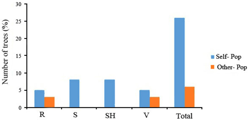
Fig. 3. Assignment percentage of individuals based on structure analysis per each population (K = 3). R = QalehRoudkhan region; S = SiyahMazgi region; SH = Shafaroud region; V = Veysroud region.

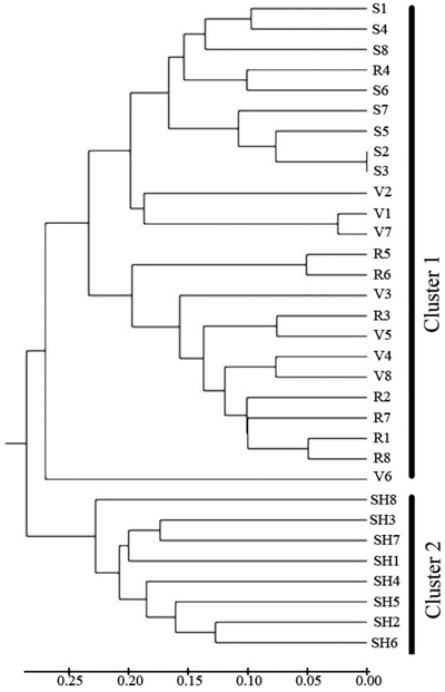
Fig. 4. Dendrogram depicting the distribution of genotypes of the four populations of C. sativa in Hyrcanian forest based on UMGMA method. R = QalehRoudkhan region; S = SiyahMazgi region; SH = Shafaroud region; V = Veysroud region.

Table 7. Results of BOTTLENECK tests elaborated on the four C. sativa populations analysed at 10 polymorphicnuclear microsatellite loci.
Test		Mutation Model	Population
Test		Mutation Model	V	SH	S	R
Sign	P-value	IAM	0.08	0.225	0.272	0.347
		SMM	0.034*	0.807	0.513	0.359
		TPM	0.072	0.359	0.335	0.369
Wilcoxon	P-value	IAM	0.359	0.921	0.496	1.000
		SMM	0.203	0.625	0.734	0.82
		TPM	0.250	0.625	0.57	0.91
Standardized differences	P-value	IAM	<0.001*	0.468	0.003*	0.396
		SMM	<0.001*	0.272	0.04*	0.057
		TPM	<0.001*	0.114	0.012	0.208
* Significant at level 0.05; P = Probability; IAM = Infinite allele model, TPM = Two phase model, SMM = Stepwise mutation model; R = QalehRoudkhan region; S = SiyahMazgi region; SH = Shafaroud region; V = Veysroud region