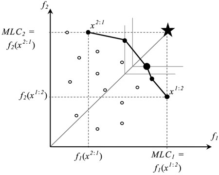
Fig. 1. A set of outcomes of feasible (○) and Pareto optimal solutions (●) of a bi-objective optimization problem. The horizontal (f1) and vertical (f2) axes correspond to biodiversity objectives 1 and 2, respectively, and x2:1 and x1:2 refer to extreme solutions corresponding to values of Maximum Landscape Capacity (MLC) (i.e., Pareto optimal outcomes). The large dot represents the Pareto optimal solution (management plan) that is closest to the ideal plan (star) where all objectives reach their maximal values. The solutions´ points are connected for visualization purposes only.
| Table 1. Management regimes applied on the forest stands (modified from Triviño et al. 2015). | ||
| Management regime | Acronym | Description |
| Business as usual | BAU | Recommended management: average rotation length 80 years; site preparation, planting or seedling trees; 1–3 thinnings; final harvest with green tree retention level 5 trees ha–1 |
| Set aside | SA | No management |
| Extended rotation (10 years) | EXT10 | BAU with postponed final harvesting by 10 years; average rotation length 90 years |
| Extended rotation (30 years) | EXT30 | BAU with postponed final harvesting by >30 years; average rotation length 115 years |
| Green tree retention | GTR30 | BAU with 30 green trees retained/ha at final harvest; average rotation length 80 years |
| No thinnings (final harvest threshold values as in BAU) | NTLR | Otherwise BAU regime but no thinnings; therefore trees grow more slowly and final harvest is delayed; average rotation length 86 years |
| No thinnings (minimum final harvest threshold values) | NTSR | Otherwise BAU regime but no thinnings; final harvest adjusted so that rotation does not prolong: average rotation length 77 years |
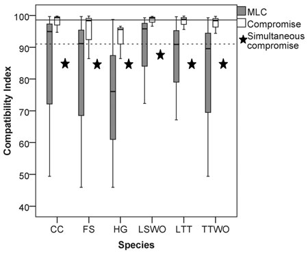
Fig. 2. Box (median and interquartile range) and whiskers (variability outside quartiles) plots show the range of compatibility index values for each species for: (grey) pairwise solutions maximizing landscape capacity for a single species (MLC), and (white) pairwise compromise solutions. Stars represent relative habitat availability under a compromise solution that simultaneously minimizes the loss of habitat for all the species, expressed in terms of % of habitat availability to MLC. The horizontal reference lines represent the median value among all the species for: (dotted line) solutions maximizing single-species landscape capacity and (continuous line) the pairwise compromise solutions. Abbreviations on the x-axis: CC = capercaillie, FS = flying squirrel, HG = hazel grouse, LTT = long-tailed tit, LSWO = lesser-spotted woodpecker, TTWO = three-toed woodpecker.
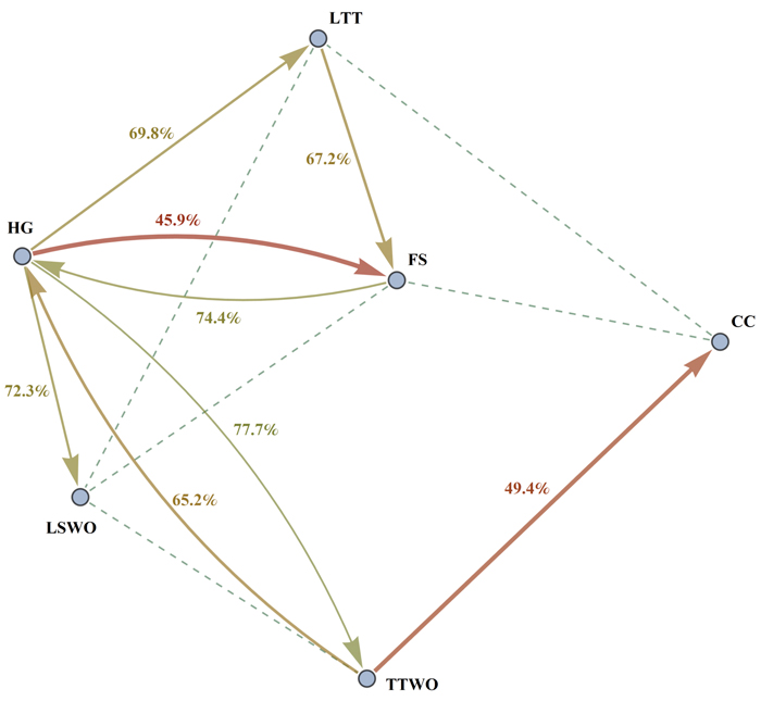
Fig. 3. Graph of compatibility indices R1(2) and R2(1) between different pairs of species. The figure shows conflicts between species as follows: an arrow from species 1 to species 2 represents the level of compatibility of the species 1 to the species 2. More intense conflicts (lower compatibility indices) are represented by thick red arrows, intermediate conflicts by thinner yellow arrows. Only conflicts with the compatibility index less than 85% are shown for better readability. Dashed lines are drawn between pairs of species which have high reciprocal compatibility index values (for which R1(2) + R2(1) ≥ 190%). Species abbreviations are as in the caption of Fig. 2.
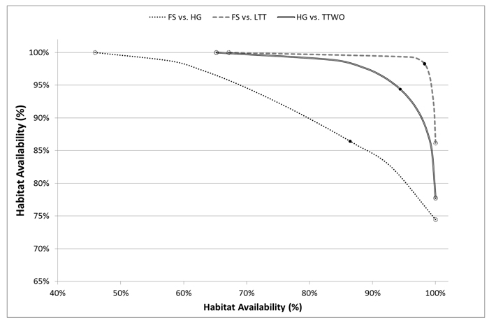
Fig. 4. Trade-off curves for habitat availability of selected pairs of species for which at least one conflict is evident (one of the two compatibility indices is low) plotted in x and y-axes. Solutions deriving from management plans maximizing landscape capacity for single species are pointed out on the curve with empty dots, compromise solutions with black dots. Species abbreviations are in the caption of Fig. 2.
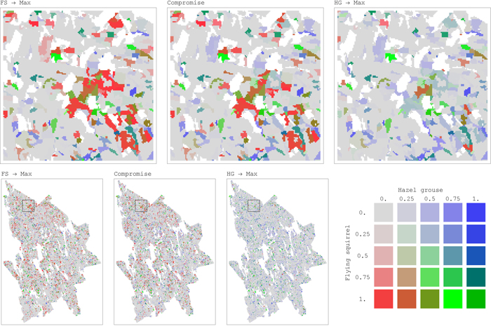
Fig. 5. Maps of distribution of habitat availability values for a pair of conflicting species, flying squirrel (FS) and hazel grouse (HG), in the study area for each forest stand (25 m × 25 m resolution) (maps on top present magnification of regions, outlined in the map at the bottom left with black square borders). Habitat Availability combinations for the two species shown in each of the three maps represent outcomes of the corresponding management plans: maximizing landscape capacity for one species only (FS → Max, HG → Max) and the compromise management plans addressing landscape capacity for both the species. The color palette is defined by the ratio between habitat availability values of the two species. The intensity of the color corresponds to the absolute values of habitat availability. Color legend: red when habitat availability of FS is positive while habitat availability of HG is zero. Blue when habitat availability of HG is positive while habitat availability of FS is zero. Green when both species’ habitat availabilities are positive and “fairly” shared between them. The “fair” share is defined as the ratio between the average values of maximum (across management regimes) habitat availability achieved for each species at each stand, where only positive habitat availability values are considered, for FS and HG these averages are 0.42 and 0.32, respectively. View larger in new window/tab
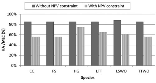
Fig. 6. Comparison of simultaneous compromise solutions for all the six species without and with money constraint. The simultaneous compromise solutions, expressed in terms of percentage Habitat Availability (HA) to Maximum Landscape Capacity (MLC), minimize the loss of habitat among all the species. The management plan obtained by the solution without NPV (Net Present Value) constraint aims at only solving conflicts among all species, the management plan with NPV constraint solves conflicts among all species while obtaining 95% of the NPV from timber extraction. Species abbreviations are in the caption of Fig. 2.