| Table 1. Parameters of the LiDAR data sets. | ||
| Scanner | Riegl LMS-Q680i | Leica ALS60 |
| Wavelength, nm | 1550 | 1064 |
| Date | May 28, 2013 | June 16, 2013 |
| Pulse repetition frequency, Hz | 240 | 106 |
| FWHM, transmitted pulse, ns | 4.5 | 7.8 |
| Pulse density p×m–2 | 12−20 | 10 |
| Flying height, m | 750 | 700 |
| Flying speed, m×s–1 | 41 | 62 |
| Strip overlap, % | 75 | 55 |
| Scan angle, ±° | 30 | 15 |
| Footprint diameter (86%), cm | 36 | 16 |
| WF samples per pulse | n × 80 | 1 × 256 |
| WF sampling rate, GHz | 1 | 1 |
| Discrete returns per pulse | 1−10 | 1−4 |
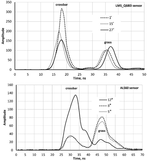
Fig. 1. Sample waveforms (WFs) of three LMS680i and three ALS60 pulses intersecting a football goal’s crossbar (height 2.5 m) and grass. The scan zenith angles (SZAs) are marked in degrees. WF sequences start with a buffer of amplitude values that display the signal prior to the storage-triggering echo. Their length is approximately 12 and 20 nanoseconds in the two sensors. The WF peaks (crossbar–grass) are separated more in the oblique pulse with an SZA of 27° compared to the vertical pulse (SZA = 1°). Return pulses of LMS-Q680i are symmetric, whereas ALS60 return pulses display ‘a tail’ even in hard targets. The asymmetry is due to the shutter in the laser transmitter that closes ‘slowly’.
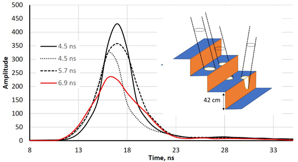
Fig. 2. Illustration of echo-widening in the LMS-Q680i. The four return waveforms are from wooden benches with a 42-cm vertical spacing. Echo widths (defined as full-width- half-maximum, FWHM) range from 4.5 ns to 6.9 ns. The width was 4.5 ns for pulses that illuminated a single planar surface. The pulse that displayed a 6.9-ns echo width intersected two bench layers, and the 5.3-ns pulse likely also illuminated the vertical part of the structure (illustrated by the drawing with three pulses).
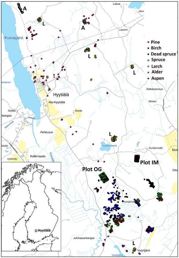
Fig. 3. Map of reference trees in Hyytiälä (61°49´N, 24°18´E), Finland. Field plots OG and IM are marked separately on the map, as well as the larch (L), and alder (A) stands. The map shows an area of 3×5 km.

Fig. 4. Stem diameter(dbh)×height distributions of trees in field plots IM and OG.

Fig. 5. Height distributions of trees measured in aerial images. Dead refers to dead spruce.
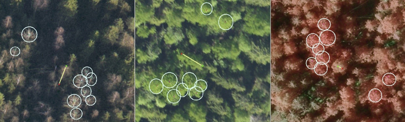
Fig. 6. Example of visual multi-image interpretation with 9 aspen crowns detected in leaf-off and leaf-on images captured in 11/2011 (left), 5/2013 (middle) and 6/2012 (right). The line segments show the ‘stem’ of a 24-m-high birch, which is used as the center point. The other ‘greyish’ trees in the leaf-off image are birches, and the green crowns are spruces.
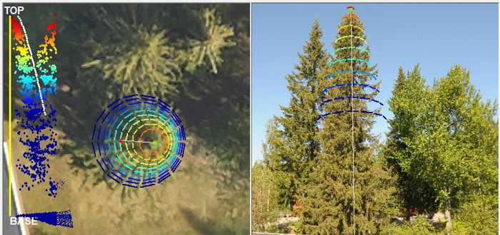
Fig. 7. Illustration of crown modeling of an urban Norway spruce. Aerial image on the left has the target tree in the middle with the current solution of the crown model superimposed as a colored wireframe graph. Terrestrial image on the right was taken from the roof of a building and was included here for illustration only. The graph in the left part of the aerial image shows the stem (yellow line) connecting the treetop and the base. The colored points are the LiDAR points near the tree. Their x-coordinate is the horizontal distance to the stem. Returns from the neighboring spruce are visible in the colored point cloud.
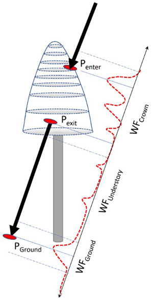
Fig. 8. Illustration of the capture of WF segments of a pulse that intersects the crown of a reference tree. Points Penter, Pexit and PGround are 3D intersection points used for splitting the entire WF between the segments. Because of convolution, the segments include amplitude values ‘before and after’ the ‘exact’ points and the segments have some overlap following Pexit and 1−2 m above the ground. WF attributes derived for the amplitude sequences are listed in Table 2.
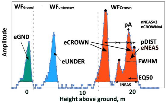
Fig. 9. An ALS60 WF of a 21.5-m-high pine. Graph illustrates the three WF segments and their WF attributes. WFCrown extends from 21 to 12 m and has four peaks (nCROWN = 4). eCROWN (crown energy) is the sum of amplitude values in WFCrown. pDist is the average distance between the peaks in WFCrown. The first-return NEAS amplitude sequence has three peaks (nNEAS = 3) and the length was 27 nanoseconds (lNEAS). The value of EQ50 is <0.5 as the NEAS energy is concentrated in the initial part. Understory energy (eUNDER) is due to the pulse intersecting the trunk or a dead branch 3−4 m above the ground. The pulse gave rise to a weak ground signal, and eGND (ground energy) is the sum of amplitude values belonging to WFGround. Echo width (FWHM) is computed using pA, which is the maximum amplitude in the NEAS.
| Table 2. WF attributes of each pulse intersecting a tree crown. Attributes marked with * were directly adopted from Hovi et al. (2016). See Fig. 8 for the definition of WF segments representing the crown, understory and ground. | |
| Attribute | Definition |
| eCROWN | Crown energy. Sum of amplitude values assigned to WFCrown |
| eNEAS* | Energy of the (first-return) noise-exceeding amplitude sequence, NEAS |
| eUNDER | Understory energy. Sum of amplitude values assigned to WFUnderstory |
| eGND | Ground energy. Sum of amplitude values assigned to WFGround |
| nCROWN | Number of local maxima in WFCrown |
| nNEAS* | Number of local maxima in the (first) NEAS |
| pA* | Maximum amplitude in the NEAS, ‘peak amplitude’ |
| FWHM* | Width of the echo giving pA, nanoseconds |
| lNEAS* | Total length of the NEAS, nanoseconds |
| pDist | Mean distance between local peaks in WFCrown, meters |
| MinRelDist | Minimum relative horizontal pulse-trunk distance inside the crown, 0−1 |
| pADist | Horizontal distance to the trunk of point pA, meters |
| pARelDist | Horizontal distance to the trunk of point pA, relative, 0−1 |
| EQ50 | Relative distance of the energy median from the start of the NEAS, 0−1 |
| SZA | Scan zenith angle, degrees |
| Table 3. Comparison of mean features by species relative to pine. Features are described in Table 2 and Fig. 9. The colors highlight the differences. Dead S refers to dead spruce. | |||||||
| Mean feature | Pine | Spruce | Birch | Aspen | Alder | Larch | Dead S |
| m_eCROWN_1064 | 100 | 120 | 136 | 140 | 165 | 135 | 86 |
| m_eUNDER_1064 | 100 | 151 | 138 | 135 | 105 | 127 | 135 |
| m_eGND_1064 | 100 | 60 | 64 | 40 | 44 | 66 | 136 |
| m_nCROWN_1064 | 100 | 103 | 108 | 109 | 104 | 106 | 117 |
| m_eNEAS_1064 | 100 | 118 | 135 | 139 | 166 | 135 | 79 |
| m_pA_1064 | 100 | 124 | 128 | 133 | 164 | 127 | 84 |
| m_nNEAS_1064 | 100 | 100 | 106 | 105 | 101 | 105 | 103 |
| m_lNEAS_1064 | 100 | 100 | 114 | 115 | 118 | 114 | 88 |
| m_FWHM_1064 | 100 | 93 | 104 | 101 | 98 | 104 | 94 |
| m_pDist_1064 | 100 | 107 | 109 | 114 | 121 | 102 | 108 |
| m_EQ50_1064 | 100 | 103 | 100 | 97 | 93 | 101 | 106 |
| m_MinRelDist_1064 | 100 | 101 | 104 | 105 | 103 | 102 | 95 |
| m_pARelDist_1064 | 100 | 93 | 103 | 106 | 112 | 104 | 90 |
| m_eCROWN_1550 | 100 | 95 | 105 | 82 | 111 | 115 | 146 |
| m_eUNDER_1550 | 100 | 125 | 106 | 102 | 95 | 119 | 198 |
| m_eGND_1550 | 100 | 86 | 88 | 68 | 80 | 86 | 114 |
| m_nCROWN_1550 | 100 | 97 | 105 | 110 | 114 | 103 | 100 |
| m_eNEAS_1550 | 100 | 92 | 105 | 77 | 109 | 115 | 142 |
| m_pA_1550 | 100 | 102 | 99 | 79 | 105 | 112 | 140 |
| m_nNEAS_1550 | 100 | 93 | 103 | 96 | 107 | 104 | 100 |
| m_lNEAS_1550 | 100 | 88 | 106 | 90 | 107 | 108 | 103 |
| m_FWHM_1550 | 100 | 96 | 104 | 106 | 106 | 105 | 98 |
| m_pDist_1550 | 100 | 99 | 105 | 109 | 110 | 99 | 101 |
| m_EQ50_1550 | 100 | 106 | 100 | 103 | 97 | 100 | 107 |
| m_MinRelDist_1550 | 100 | 98 | 103 | 106 | 105 | 102 | 85 |
| m_pARelDist_1550 | 100 | 92 | 103 | 107 | 111 | 105 | 78 |
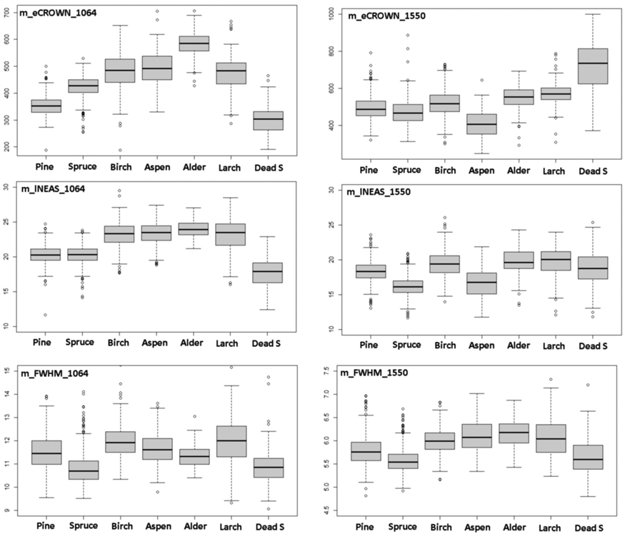
Fig. 10. Comparison of 1064-nm and 1550-nm features m_eCROWN, m_lNEAS and m_FWHM by species. Features are described in Table 2 and Fig. 9. View larger in new window/tab.
| Table 4. Correlation of mean waveform features with tree height by wavelength (1064, 1550) and species. Features are described in Table 2 and Fig. 9. The colors highlight the differences. Dead S refers to dead spruce. | ||||||||||||||||
| 1064 | 1550 | 1064 | 1550 | 1064 | 1550 | 1064 | 1550 | 1064 | 1550 | 1064 | 1550 | 1064 | 1550 | 1064 | 1550 | |
| All | Pine | Spruce | Birch | Aspen | Alder | Larch | Dead S | |||||||||
| m_eCROWN | 0.01 | 0.30 | 0.40 | 0.66 | 0.36 | 0.53 | –0.22 | –0.23 | 0.01 | 0.17 | 0.10 | 0.06 | –0.44 | 0.21 | 0.30 | 0.42 |
| s_eCROWN | –0.01 | 0.23 | 0.34 | 0.63 | –0.04 | 0.33 | –0.15 | –0.20 | 0.19 | 0.17 | 0.15 | 0.16 | –0.14 | 0.42 | –0.21 | 0.12 |
| m_eUNDER | –0.07 | 0.07 | 0.14 | 0.22 | 0.04 | 0.13 | –0.29 | –0.18 | –0.23 | –0.36 | –0.14 | 0.14 | –0.29 | –0.19 | 0.17 | 0.24 |
| s_eUNDER | 0.02 | 0.14 | 0.16 | 0.23 | 0.27 | 0.29 | –0.23 | –0.06 | –0.09 | –0.12 | –0.18 | –0.13 | –0.25 | –0.16 | 0.25 | 0.28 |
| m_eGND | –0.22 | –0.06 | –0.36 | –0.20 | –0.41 | –0.11 | –0.28 | –0.13 | 0.00 | 0.04 | –0.57 | –0.51 | 0.13 | 0.30 | –0.59 | –0.33 |
| s_eGND | –0.10 | –0.05 | –0.27 | –0.05 | –0.16 | –0.18 | –0.11 | 0.04 | 0.18 | 0.02 | –0.50 | –0.30 | 0.18 | 0.23 | –0.48 | –0.24 |
| m_nCROWN | 0.39 | 0.50 | 0.18 | 0.31 | 0.51 | 0.70 | 0.40 | 0.44 | 0.23 | 0.62 | 0.26 | 0.40 | 0.45 | 0.65 | 0.52 | 0.56 |
| s_nCROWN | 0.44 | 0.60 | 0.21 | 0.51 | 0.57 | 0.72 | 0.48 | 0.56 | 0.39 | 0.70 | 0.31 | 0.50 | 0.41 | 0.66 | 0.48 | 0.63 |
| m_eNEAS | –0.05 | 0.17 | 0.31 | 0.55 | 0.17 | 0.31 | –0.27 | –0.36 | –0.03 | 0.04 | 0.04 | –0.09 | –0.47 | –0.11 | 0.20 | 0.23 |
| s_eNEAS | 0.09 | 0.25 | 0.43 | 0.63 | 0.27 | 0.41 | –0.08 | –0.25 | 0.24 | 0.09 | 0.21 | 0.08 | –0.07 | 0.47 | 0.05 | 0.22 |
| m_pA | 0.00 | 0.26 | 0.48 | 0.63 | 0.29 | 0.44 | –0.24 | –0.26 | 0.00 | 0.04 | 0.03 | –0.11 | –0.30 | 0.17 | 0.15 | 0.19 |
| s_pA | 0.11 | 0.29 | 0.44 | 0.54 | 0.45 | 0.55 | –0.03 | –0.06 | 0.18 | 0.09 | 0.07 | –0.12 | –0.16 | 0.30 | 0.05 | 0.15 |
| m_nNEAS | 0.05 | 0.11 | –0.22 | –0.25 | 0.07 | 0.26 | 0.11 | –0.09 | –0.08 | 0.14 | 0.04 | 0.10 | 0.01 | 0.02 | 0.30 | 0.42 |
| s_nNEAS | 0.11 | 0.23 | –0.19 | –0.12 | 0.16 | 0.33 | 0.18 | 0.07 | 0.06 | 0.23 | 0.05 | 0.23 | 0.07 | 0.28 | 0.32 | 0.49 |
| m_lNEAS | –0.05 | 0.02 | –0.24 | –0.27 | 0.01 | 0.08 | –0.07 | –0.24 | –0.02 | 0.08 | 0.08 | –0.04 | –0.44 | –0.29 | 0.30 | 0.34 |
| s_lNEAS | 0.15 | 0.26 | –0.10 | –0.09 | 0.16 | 0.37 | 0.20 | 0.01 | 0.23 | 0.28 | 0.24 | 0.29 | 0.24 | 0.54 | 0.29 | 0.43 |
| m_FWHM | –0.24 | –0.23 | –0.50 | –0.44 | –0.43 | –0.40 | –0.18 | –0.10 | –0.20 | –0.06 | –0.06 | –0.30 | –0.44 | –0.51 | 0.08 | –0.25 |
| s_FWHM | –0.01 | –0.16 | –0.11 | –0.34 | –0.07 | –0.21 | 0.03 | –0.05 | 0.08 | –0.13 | –0.12 | –0.15 | 0.00 | –0.45 | 0.02 | –0.09 |
| m_pDist | 0.50 | 0.55 | 0.61 | 0.71 | 0.63 | 0.63 | 0.55 | 0.63 | 0.46 | 0.62 | 0.42 | 0.41 | 0.48 | 0.69 | 0.28 | 0.31 |
| s_pDist | 0.52 | 0.50 | 0.58 | 0.63 | 0.61 | 0.58 | 0.51 | 0.51 | 0.41 | 0.51 | 0.32 | 0.32 | 0.46 | 0.49 | 0.35 | 0.24 |
| m_EQ50 | –0.24 | –0.21 | –0.43 | –0.42 | –0.32 | –0.31 | –0.35 | –0.12 | –0.29 | –0.20 | –0.15 | 0.06 | –0.35 | –0.06 | 0.03 | –0.17 |
| s_EQ50 | –0.09 | 0.00 | –0.08 | 0.05 | –0.10 | 0.00 | –0.05 | –0.01 | –0.23 | –0.03 | –0.12 | –0.09 | –0.18 | 0.11 | 0.25 | 0.11 |
| m_MinRelDist | –0.07 | –0.14 | –0.25 | –0.33 | –0.02 | –0.15 | –0.07 | –0.05 | 0.02 | –0.13 | –0.09 | –0.24 | –0.23 | –0.31 | 0.22 | 0.09 |
| s_MinRelDist | 0.07 | 0.12 | 0.08 | 0.16 | 0.11 | 0.21 | 0.01 | 0.23 | –0.11 | –0.21 | –0.50 | –0.07 | –0.09 | –0.05 | 0.14 | 0.12 |
| m_pARelDist | 0.30 | 0.23 | 0.36 | 0.33 | 0.37 | 0.31 | 0.48 | 0.45 | 0.26 | 0.27 | 0.01 | 0.16 | 0.25 | 0.34 | 0.32 | 0.23 |
| s_pARelDist | –0.14 | –0.08 | –0.27 | –0.13 | –0.30 | –0.15 | 0.06 | 0.11 | –0.16 | –0.25 | –0.12 | –0.06 | –0.03 | –0.10 | –0.29 | –0.07 |
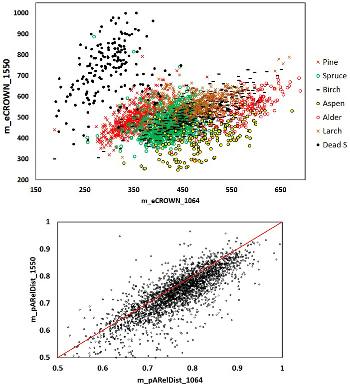
Fig. 11. 1064 and 1550 nm mean crown energy and mean relative distance of the strongest return from the trunk in 2532 trees. Dead spruce separates well in eCROWN_1064 and eCROWN_1550. Some of the outliers may be due to species errors in the field data or in image interpretation. The asymmetry of the m_pARelDist point pattern shows how the strongest echoes of 1550-nm pulses (36 cm footprint diameter) have reflected from farther off the stem compared to 1064-nm pulses (16 cm). Features are described in Table 2 and Fig. 9.
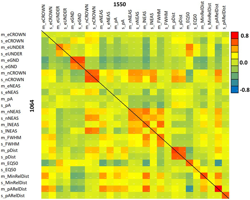
Fig. 12. Correlation between 1064 and 1550 nm features. The diagonal elements show the between-wavelength correlation of the same feature. Features are described in Table 2 and Fig. 9.
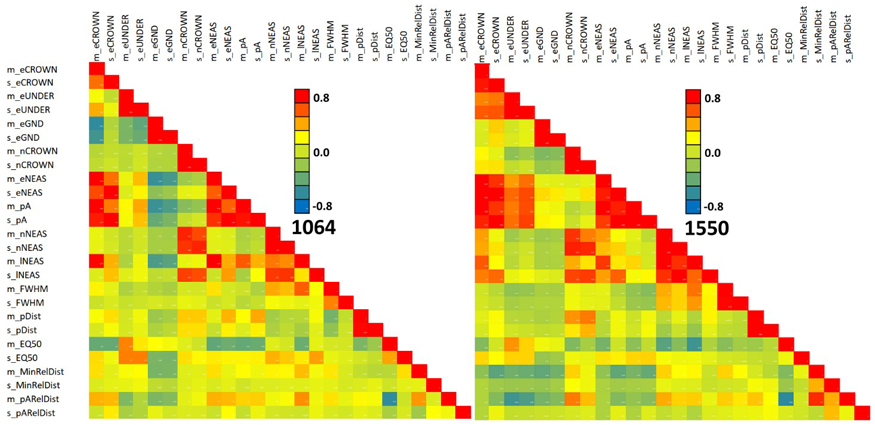
Fig. 13. Correlation of 1064 and 1550 nm features in all trees. Features are described in Table 2 and Fig. 9. View larger in new window/tab.
| Table 5. Average overall accuracy (OA,%) and kappa in QDA classifications using repeated (n = 1000) random sub-sampling validation with random splits between training and validation data using ratios 100:100, 90:10, 80:20, 50:50 and 20:80. Case 100:100 was computed only once and represents an optimistic scenario. Classification was done using 7, 6, 4 and 3 species classes using ten WF features ranked by F-test or Gini-importance. Only the range is given for kappa, not the values of all five validation scenarios. | |||||
| Classes | Wavelength | OA % with F-test variables | OA (%) with Gini-variables | F-test | Gini-vars |
| 100 90 80 50 20% | 100 90 80 50 20% | kappa | kappa | ||
| All seven | 1064 | 76.7 73.5 73.3 72.5 69.9 | 76.7 73.6 73.3 72.5 69.8 | 0.711→0.624 | 0.711→0.624 |
| 1550 | 78.1 76.0 75.9 75.6 73.3 | 80.3 78.1 77.9 77.5 75.1 | 0.729→0.669 | 0.756→0.691 | |
| 1064+1550 | 84.1 83.0 82.7 82.3 79.9 | 86.5 84.7 84.6 84.0 81.5 | 0.802→0.750 | 0.833→0.801 | |
| 6 classes, without larch | 1064 | 83.5 80.9 80.6 80.1 77.6 | 83.5 80.8 80.7 80.1 77.6 | 0.785→0.706 | 0.785→0.706 |
| 1550 | 83.2 81.6 81.6 81.0 79.1 | 84.0 82.3 82.4 81.7 79.5 | 0.783→0.727 | 0.793→0.732 | |
| 1064+1550 | 88.7 87.9 87.8 87.4 85.5 | 91.3 90.0 90.1 89.7 87.6 | 0.855→0.810 | 0.889→0.838 | |
| 4 classes, pine, spruce, birch, dead spruce | 1064 | 88.7 87.6 87.6 87.3 86.1 | 88.7 87.7 87.7 87.4 86.1 | 0.838→0.800 | 0.838→0.800 |
| 1550 | 88.2 87.3 87.2 86.8 85.7 | 89.0 88.1 88.1 87.8 86.7 | 0.831→0.795 | 0.842→0.809 | |
| 1064+1550 | 91.1 90.6 90.6 90.4 89.6 | 93.5 92.7 92.7 92.6 91.8 | 0.871→0.850 | 0.906→0.881 | |
| 3 classes, pine, spruce, birch | 1064 | 90.8 89.8 89.7 89.5 88.4 | 90.8 89.9 89.8 89.5 88.4 | 0.855→0.819 | 0.855→0.817 |
| 1550 | 88.7 87.9 87.6 87.1 85.9 | 89.2 88.4 88.4 88.0 86.8 | 0.824→0.780 | 0.830→0.793 | |
| 1064+1550 | 91.6 91.2 91.1 90.8 89.9 | 93.9 93.5 93.3 93.0 92.2 | 0.868→0.841 | 0.905→0.878 | |
| Table 6. Average confusion matrix in 1000 randomized validations using 80% of the trees for training and 20% for validation. The predictors were the five best 1064 and 1550 nm features by Gini-importance (Kappa = 0.808, OA = 84.6%). Dead refers to dead spruce. | |||||||
| QDA class | True class | ||||||
| Pine | Spruce | Birch | Aspen | Alder | Larch | Dead | |
| Pine | 436 | 19 | 9 | 10 | 4 | ||
| Spruce | 38 | 741 | 15 | 2 | 47 | 6 | |
| Birch | 4 | 13 | 328 | 23 | 13 | 60 | 1 |
| Aspen | 1 | 12 | 129 | 9 | 3 | ||
| Alder | 10 | 10 | 125 | 1 | |||
| Larch | 7 | 13 | 44 | 3 | 241 | ||
| Dead | 7 | 11 | 2 | 175 | |||
| Table 7. Average Producer’s accuracy (%) by species in classifications of seven species classes using predictors selected by Gini-importance (90:10 ratio of training and validation). Dead refers to dead spruce. | |||||||
| Wavelenght | Pine | Spruce | Birch | Aspen | Alder | Larch | Dead |
| 1064 nm | 87 | 85 | 51 | 46 | 78 | 61 | 79 |
| 1550 nm | 78 | 88 | 68 | 67 | 58 | 76 | 90 |
| 1064+1550 nm | 91 | 87 | 75 | 84 | 86 | 79 | 89 |
| Table 8. Feature ranking by F-test and Gini-importance in data combining all seven species. 1064 and 1550 refer to the wavelength. Features are described in Table 2 and Fig. 9. | |||
| F-test 1064 | F-test 1550 | Gini 1064 | Gini 1550 |
| m_eCROWN | s_eNEAS | m_lNEAS | m_lNEAS |
| m_eNEAS | s_eCROWN | m_eCROWN | s_pA |
| m_pA | m_eCROWN | s_pA | s_eNEAS |
| s_pA | m_eNEAS | m_eNEAS | m_pDist* |
| s_eNEAS | s_eUNDER* | m_pA | m_FWHM |
| m_lNEAS | m_pARelDist | m_FWHM | s_eCROWN |
| s_eCROWN | s_pA | s_eNEAS | m_eNEAS |
| m_pARelDist | m_eUNDER* | s_eCROWN | m_EQ50* |
| m_EQ50 | m_lNEAS | m_EQ50 | m_pARelDist |
| m_FWHM | m_pA* | m_pARelDist | m_eCROWN |