
Fig. 1. A map of Finland and location of study area of forest attractiveness in Ruunaa area in Lieksa, eastern Finland.
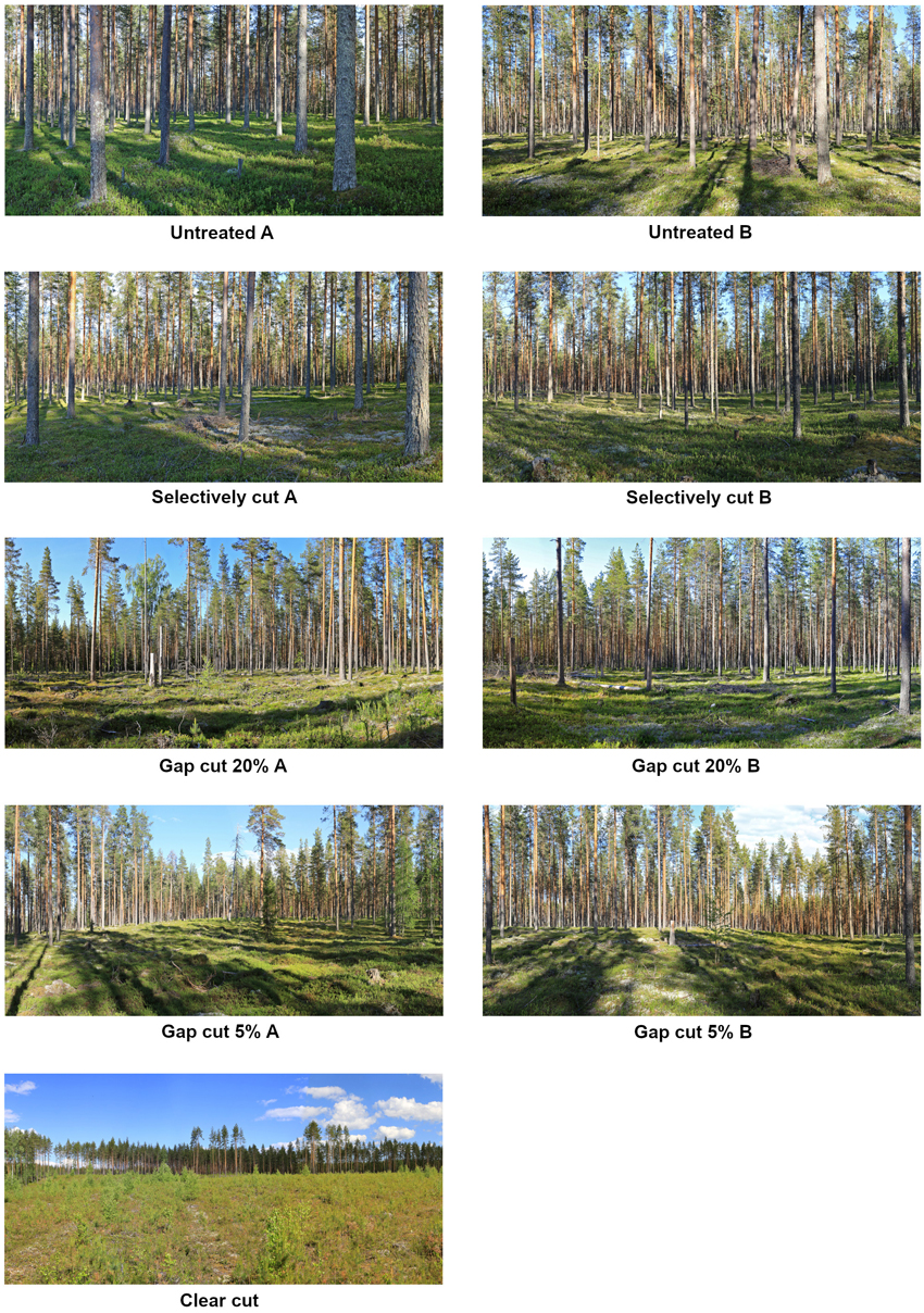
Fig. 2. Evaluated Scots pine dominated Vaccinium-type forest views in panorama images including two replicate sites which were unharvested (control, basal area 26 m2 ha–1), a selective cutting site (basal area 18 m2 ha–1), small openings sites (gap cut) with 20 and 5% retained trees, respectively, and one site which was clear cut with 3% retained trees.
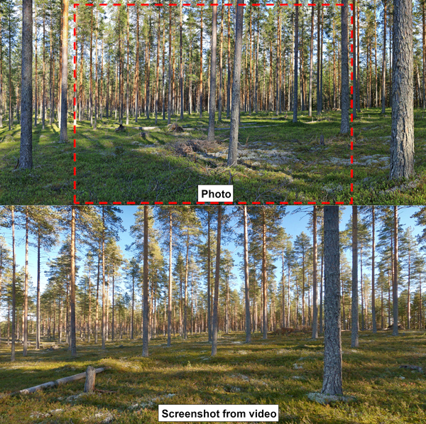
Fig. 3. Example photo and video views used in our study (selective cut). Standard photo size cropped with a red dotted line from a panoramic image.
| Table 1. Evaluation event of measuring forest attractiveness: grouping variables related to the evaluation event and methods (% of respondents). | ||
| Grouping variable: | Category: | |
| To evaluate this number of photos and videos *) | Moderately or very effortless | 51.4 |
| The evaluation of attractiveness in general *) | Moderately or very easy | 52.9 |
| Photos contra videos (the easy of evaluations): *) | Easier from the photos | 17.1 |
| Easier from the videos | 27.1 | |
| Equally easy | 55.7 | |
| Imagining the forest from the photos *) | Well or very well | 75.7 |
| Imagining the forest from the videos *) | Well or very well | 84.3 |
| The quality of the images was good | Yes | 100 |
| The quality of the videos was good | Yes | 95.8 |
| The time of looking photos was | Too long | 5.7 |
| About right | 91.4 | |
| Too short | 2.9 | |
| The length of the videos was | Too long | 41.4 |
| About right | 55.7 | |
| Too short | 2.9 | |
| The vertical motion in the videos: *) | Positive | 40.0 |
| Neutral | 50.0 | |
| Negative | 10.0 | |
| The poorer quality of images and videos would have affected to the evaluation *) | Yes | 56.3 |
| Noises (e.g., birds and wind) would have affected to the evaluation *) | Yes | 53.5 |
| Particular attention to the forest floor *) | Yes | 45.7 |
| Particular attention to the trees *) | Yes | 54.2 |
| *) Involved in group analyses according to the grouping presented here. | ||
| Table 2. Statistical differences in forest attraction between visualization methods: entire data and treatments. Significant < 0.01 in bold and significance 0.01–0.05 in italic and underscore. | |||||
| Treatment: | F | p | Contrast: | F | p |
| Average of all treatments | 19.992 | <0.001 | Video vs. Photo | 25.465 | <0.001 |
| Video vs. Panorama | 24.336 | <0.001 | |||
| Photo vs. Panorama | 0.119 | 0.731 | |||
| Untreated | 16.722 | <0.001 | Video vs. Photo | 22.863 | <0.001 |
| Video vs. Panorama | 17.719 | <0.001 | |||
| Photo vs. Panorama | 2.490 | 0.119 | |||
| Selectively cut | 18.601 | <0.001 | Video vs. Photo | 25.909 | <0.001 |
| Video vs. Panorama | 20.132 | <0.001 | |||
| Photo vs. Panorama | 1.508 | 0.224 | |||
| Gap cut 20% | 3.071 | 0.054 | |||
| Gap cut 5% | 4.018 | 0.021 | Video vs. Photo | 3.660 | 0.060 |
| Video vs. Panorama | 7.456 | 0.008 | |||
| Photo vs. Panorama | 0.391 | 0.534 | |||
| Clear cut | 4.059 | 0.029 | Video vs. Photo | 2.599 | 0.111 |
| Video vs. Panorama | 6.532 | 0.013 | |||
| Photo vs. Panorama | 1.880 | 0.175 | |||
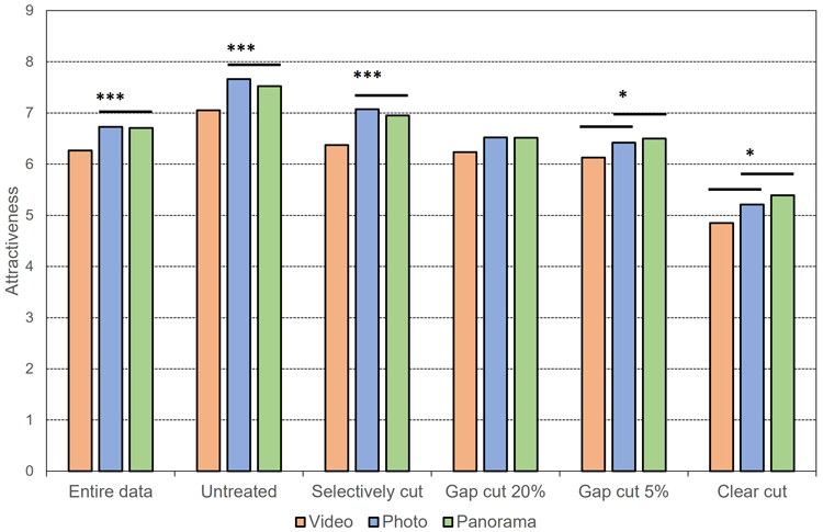
Fig. 4. Statistical differences in forest attraction between visualization methods: entire data and treatments. Equal line connects methods that did not differ statistically from each other (variance analysis of repetition measurements). Statistical significance: * < 0.05; ** < 0.01; *** < 0.001. Forest treatments presented in the Fig. 2 caption.
| Table 3. Statistical differences in forest attraction between visualization methods in group and pair comparisons: entire data and treatments. Presentation methods: V = Video; Ph = Photo; Pa = Panorama. Significant < 0.01 in bold and significance 0.01–0.05 in italic and underscore. | ||||||
| Grouping factor | Treatment | Group * Method | Contrasts of Interaction | |||
| F | p | Contrast | F | p | ||
| Easiness of assessing attractiveness | Entire data | 5.847 | 0.005 | V vs. Ph | 4.294 | 0.042 |
| V vs. Pa | 9.955 | 0.002 | ||||
| Ph vs. Pa | 1.625 | 0.207 | ||||
| Untreated | 3.644 | 0.033 | V vs. Ph | 4.576 | 0.036 | |
| V vs. Pa | 4.816 | 0.032 | ||||
| Ph vs. Pa | 0.110 | 0.741 | ||||
| Selectively cut | 3.772 | 0.030 | V vs. Ph | 1.242 | 0.269 | |
| V vs. Pa | 7.106 | 0.010 | ||||
| Ph vs. Pa | 3.406 | 0.069 | ||||
| Gap cut 5% | 3.619 | 0.031 | V vs. Ph | 1.237 | 0.270 | |
| V vs. Pa | 7.930 | 0.006 | ||||
| Ph vs. Pa | 2.528 | 0.117 | ||||
| The easiness of methods | Entire data | 3.123 | 0.020 | V vs. Ph | 3.813 | 0.027 |
| V vs. Pa | 3.846 | 0.026 | ||||
| Ph vs. Pa | 0.474 | 0.624 | ||||
| Untreated | 3.206 | 0.017 | V vs. Ph | 4.101 | 0.021 | |
| V vs. Pa | 3.367 | 0.040 | ||||
| Ph vs. Pa | 1.250 | 0.293 | ||||
| Selectively cut | 4.295 | 0.003 | V vs. Ph | 6.570 | 0.002 | |
| V vs. Pa | 3.157 | 0.049 | ||||
| Ph vs. Pa | 2.205 | 0.118 | ||||
| Gap cut 20% | 2.549 | 0.045 | V vs. Ph | 2.298 | 0.108 | |
| V vs. Pa | 3.592 | 0.033 | ||||
| Ph vs. Pa | 1.046 | 0.357 | ||||
| Particular attention to undergrowth | Entire data | 5.564 | 0.006 | V vs. Ph | 6.028 | 0.017 |
| V vs. Pa | 8.067 | 0.006 | ||||
| Ph vs. Pa | 0.152 | 0.697 | ||||
| Untreated | 4.382 | 0.017 | V vs. Ph | 5.093 | 0.027 | |
| V vs. Pa | 6.477 | 0.013 | ||||
| Ph vs. Pa | 0.009 | 0.925 | ||||
| Selectively cut | 3.738 | 0.031 | V vs. Ph | 0.489 | 0.487 | |
| V vs. Pa | 6.664 | 0.012 | ||||
| Ph vs. Pa | 5.626 | 0.021 | ||||
| Gap cut 20% | 3.592 | 0.033 | V vs. Ph | 3.275 | 0.075 | |
| V vs. Pa | 5.349 | 0.024 | ||||
| Ph vs. Pa | 0.880 | 0.352 | ||||
| Table 4. Statistical differences in forest attraction between visualization methods in intragroup comparisons: entire data and treatments. Presentation methods: V = Video; Ph = Photo; Pa = Panorama. Significant < 0.01 in bold and significance 0.01–0.05 in italic and underscore. | |||||||
| Treatment | Contrast | Easiness of assessing attractiveness | |||||
| Moderately or very easy | Less easy | ||||||
| t | p | t | p | ||||
| Entire data | V vs. Ph | 2.091 | 0.044 | 5.994 | <0.001 | ||
| V vs. Pa | 1.707 | 0.096 | 5.363 | <0.001 | |||
| Ph vs. Pa | 1.168 | 0.251 | 0.630 | 0.533 | |||
| Untreated | V vs. Ph | 2.042 | 0.049 | 4.784 | <0.001 | ||
| V vs. Pa | 1.635 | 0.111 | 4.155 | <0.001 | |||
| Ph vs. Pa | 0.988 | 0.330 | 1.359 | 0.184 | |||
| Selectively cut | V vs. Ph | 2.953 | 0.006 | 4.201 | <0.001 | ||
| V vs. Pa | 1.467 | 0.151 | 5.184 | <0.001 | |||
| Ph vs. Pa | 2.577 | 0.014 | 0.380 | 0.707 | |||
| Gap cut 5% | V vs. Ph | 0.567 | 0.574 | 2.059 | 0.048 | ||
| V vs. Pa | 0.086 | 0.932 | 3.479 | 0.001 | |||
| Ph vs. Pa | 0.666 | 0.509 | 1.507 | 0.142 | |||
| Treatment | Contrast | The easiness of methods | |||||
| Easier from the photos | Easier from the videos | Equally easy | |||||
| t | p | t | p | t | p | ||
| Entire data | V vs. Ph | 4.720 | 0.001 | 3.416 | 0.003 | 2.457 | 0.019 |
| V vs. Pa | 3.398 | 0.006 | 3.130 | 0.006 | 2.410 | 0.021 | |
| Ph vs. Pa | 0.621 | 0.547 | 0.628 | 0.538 | 0.708 | 0.483 | |
| Untreated | V vs. Ph | 3.680 | 0.004 | 3.024 | 0.007 | 2.100 | 0.042 |
| V vs. Pa | 2.207 | 0.050 | 3.474 | 0.003 | 1.652 | 0.107 | |
| Ph vs. Pa | 1.287 | 0.224 | 0.317 | 0.755 | 1.160 | 0.253 | |
| Selectively cut | V vs. Ph | 4.072 | 0.002 | 3.456 | 0.003 | 2.476 | 0.018 |
| V vs. Pa | 3.500 | 0.005 | 2.891 | 0.010 | 1.957 | 0.058 | |
| Ph vs. Pa | 2.493 | 0.030 | 0.403 | 0.692 | 0.796 | 0.431 | |
| Gap cut 20% | V vs. Ph | 2.930 | 0.014 | 1.102 | 0.285 | 0.864 | 0.393 |
| V vs. Pa | 2.449 | 0.032 | 1.481 | 0.156 | 0.157 | 0.876 | |
| Ph vs. Pa | 0.484 | 0.638 | 1.022 | 0.320 | 1.000 | 0.324 | |
| Treatment | Contrast | Particular attention to undergrowth | |||||
| Yes | No | ||||||
| t | p | t | p | ||||
| Entire data | V vs. Ph | 1.744 | 0.091 | 5.495 | <0.001 | ||
| V vs. Pa | 1.313 | 0.199 | 5.747 | <0.001 | |||
| Ph vs. Pa | 0.631 | 0.533 | 0.100 | 0.921 | |||
| Untreated | V vs. Ph | 1.681 | 0.103 | 4.863 | <0.001 | ||
| V vs. Pa | 1.169 | 0.251 | 4.304 | <0.001 | |||
| Ph vs. Pa | 1.000 | 0.325 | 1.339 | 0.189 | |||
| Selectively cut | V vs. Ph | 2.483 | 0.019 | 4.946 | <0.001 | ||
| V vs. Pa | 0.975 | 0.337 | 6.533 | <0.001 | |||
| Ph vs. Pa | 2.436 | 0.021 | 0.666 | 0.510 | |||
| Gap cut 20% | V vs. Ph | 0.395 | 0.696 | 2.675 | 0.011 | ||
| V vs. Pa | 0.431 | 0.669 | 2.701 | 0.010 | |||
| Ph vs. Pa | 1.027 | 0.313 | 0.397 | 0.694 | |||
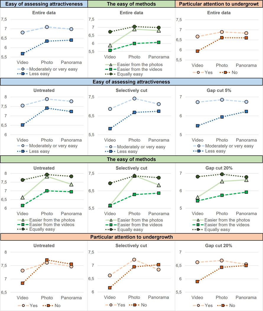
Fig. 5. The visualization method averages with groupings that showed a statistical difference in forest attraction (y-axis). At the top side by side are the groups that had statistical significant differences in the entire data. Below them are the statistical significant differences that those groups had with different forest treatments. Statistical significant differences between groups in Table 3 and internal in Table 4. Forest treatments presented in the Fig. 2. caption.
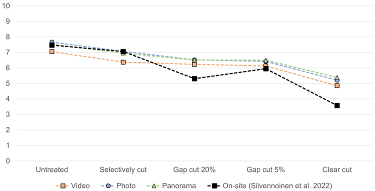
Fig. 6. Attractiveness of forest stands (y-axis) by various presentation methods (video, photo, panorama, and field assessment). Field assessment carried out in 2017 on the same forests but with a different person (Silvennoinen et al. 2022). Forest treatments presented in the Fig. 2 caption.