Silva Fennica

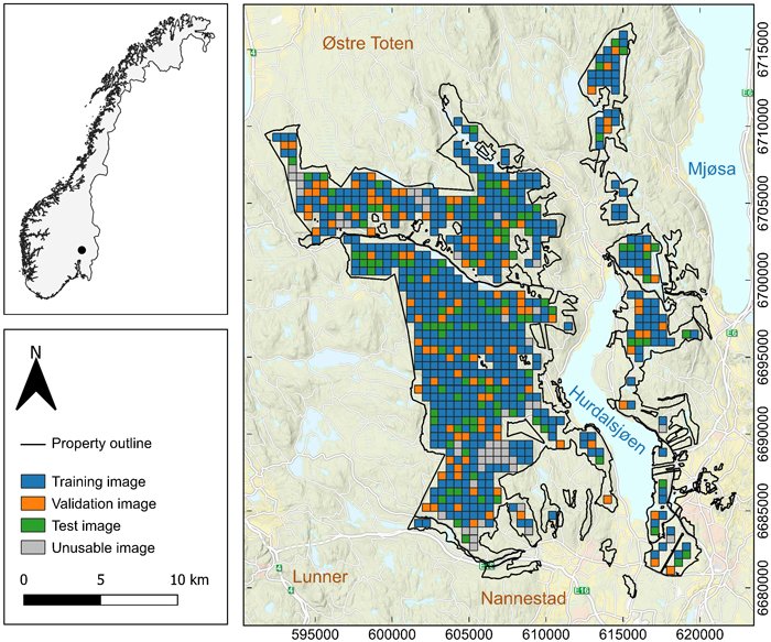
Fig. 1. Map of the forests of Mathiesen Eidsvold Værk ANS located in Akershus County, Norway. The area was divided into images tiles of 512 m × 512 m.

Table 1. Forest stand characteristics from the stand database created during the 2021 forest management planning inventory.
Class¹	Stands (n)	Area (ha)	Mean age	Volume (%)			Lorey’s mean height (m)
Class¹	Stands (n)	Area (ha)	Mean age	Spruce	Pine	Broadleaves	Min	Max	Mean
NF	3079	5159	-	-	-	-	-	-	-
I	260	538	0	-	-	-	0.0	22.0	0.4
II	1966	4799	15	-	-	-	0.1	20.0	2.3
III	2828	10 803	44	90	2	8	5.1	23.3	13.4
IV	2302	6563	68	89	2	9	6.5	25.4	16.2
V	2889	7938	101	91	3	6	6.4	28.5	18.7
¹ NF – non-forest, I-V – stand development stages.

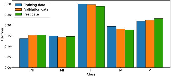
Fig. 2. Fraction of pixels across the five classes (NF – non-forest, I-II – V development stages) for each of the datasets used in model development and evaluation.

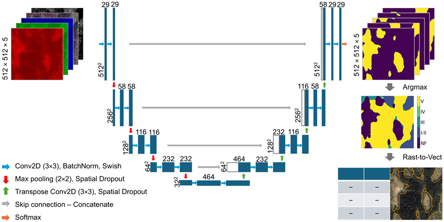
Fig. 3. Model architecture and flow of images through the model. Each blue box represents multi-channel feature maps produced by the model. The numbers along the vertical axis indicate the spatial dimensions of the images. The number of channels in the feature maps are denoted by the number on top of each box (Ronneberger et al. 2015).

Table 2. Hyperparameters and search intervals as input to Optuna.
Hyperparameter	Data type	Interval
Model parameters
Number of filters	Int	[8, 32]
Filter size	Int	[3, 7]
Learning rate	Float	[0.00001, 0.001]
Dropout rate	Float	[0.0, 0.5]
Loss parameters
Alpha	Float	[0.3, 0.7]
Beta	Float	1 – alpha
Gamma	Float	[1, 3]

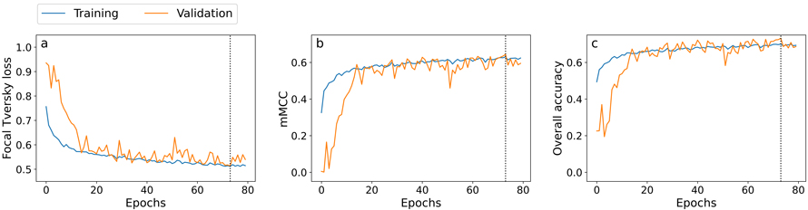
Fig. 4. Training history for the best performing model, showing development of the focal Tversky loss, mMCC, and overall accuracy for both training (blue) and validation (orange) data over 80 epochs. A dotted vertical line marks the best epoch, at which the model was automatically saved by Weights & Biases.

Table 3. Normalized confusion matrix comparing the predicted mask with the reference masks in the test data. Each cell gives the proportion relative to the total number of pixels being evaluated. The detected and correctly classified pixels (TP) are represented by the bold elements along the diagonal of the shaded area. Producer’s accuracy (PA) and user’s accuracy (UA) are calculated for each class, giving insights into omission and commission errors.
		Reference					Sum	UA
		NF	I-II	III	IV	V	Sum	UA
Predicted	NF	0.12	0.00	0.01	0.01	0.01	0.14	0.85
	I-II	0.00	0.11	0.01	0.00	0.00	0.13	0.84
	III	0.02	0.02	0.21	0.03	0.01	0.29	0.73
	IV	0.00	0.00	0.05	0.10	0.02	0.18	0.55
	V	0.01	0.01	0.01	0.05	0.18	0.26	0.70
	Sum	0.15	0.15	0.29	0.18	0.23	1
	PA	0.78	0.75	0.73	0.55	0.79

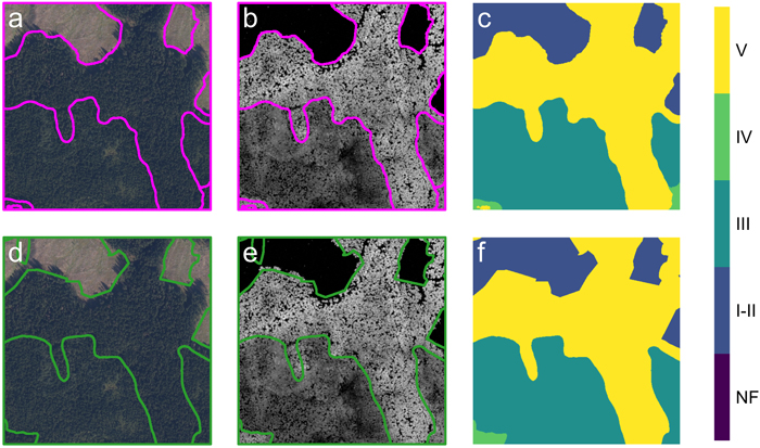
Fig. 5. Model prediction and corresponding reference data for Example 1. (a-c) Model prediction results: (a) delineated boundaries overlaid on the RGB image, (b) boundaries overlaid on the canopy height model, and (c) predicted classification mask. (d-f) Reference data: (d) annotated boundaries overlaid on the RGB image, (e) boundaries overlaid on the canopy height model, and (f) reference classification mask. Class labels: NF – non-forest, I-II - V – development stage.

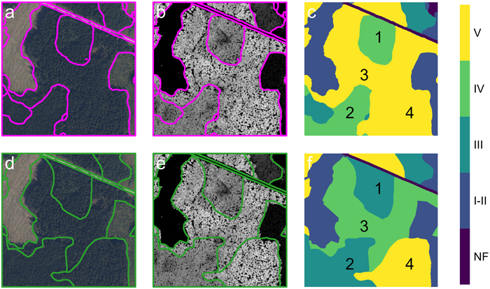
Fig. 6. Model prediction and corresponding reference data for Example 2. (a-c) Model prediction results: (a) predicted boundaries overlaid on the RGB image, (b) boundaries overlaid on the canopy height model, and (c) predicted classification mask. (d-f) Reference data: (d) annotated boundaries overlaid on the RGB image, (e) boundaries overlaid on the canopy height model, and (f) reference classification mask. Class labels: NF – non-forest, I-II - V – development stage. Numbered regions (1-4) highlights classification nuances: regions 1 and 2 show stands with ages near the transition between classes III and IV; regions 3 and 4 show where the model has merged two neighboring stands into a single operational unit.

Table 4. Stand characteristics for stands 3 and 4.
Attribute	Stand 3	Stand 4
Class	IV	V
Age	67	82
Site index (H₄₀)	G20	G20
Tree species composition¹ (S, P, B)	(99, 0, 1)	(100, 0, 0)
Volume (m³ ha^–1)	462.0	497.2
Height (m)	23.6	24.5
Basal area (m² ha^–1)	46	48
Mean diameter (cm)	26.3	27.4
¹ Percentage distribution of spruce (S), pine (P), and broadleaves (B)

Fig. 7. Model prediction and corresponding reference data for Example 2. (a-c) Model prediction results: (a) predicted boundaries overlaid on the RGB image, (b) boundaries overlaid on the canopy height model, and (c) predicted classification mask. (d-f) Reference data: (d) annotated boundaries overlaid on the RGB image, (e) boundaries overlaid on the canopy height model, and (f) reference classification mask. Class labels: NF – non-forest, I-II - V – development stage.