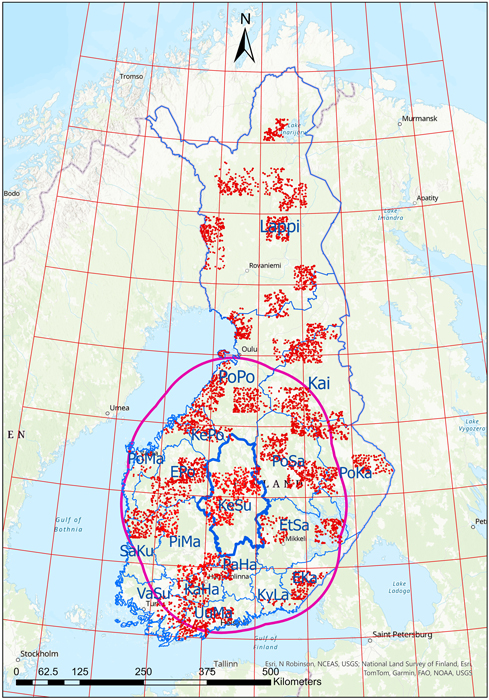
Fig. 1. The forestry districts of Finland (delineated in blue), shown with climate data zones overlaid (red grid). The solid magenta line shows an example of the climate data zones (red grid) within 150 km of the Keski-Suomi (KeSu) forestry district border. The field inventory plot locations shown with red dots. EKa = Etelä-Karjala, EPo = Etelä-Pohjanmaa, EtSa = Etelä-Savo, KaHa = Kanta-Häme, Kai = Kainuu, KePo = Keski-Pohjanmaa, KeSu = Keski-Suomi, KyLa = Kymenlaakso, Lappi = Lappi, PaHa = Päijät-Häme, PiMa = Pirkanmaa, PoKa = Pohjois-Karjala, PoMa = Pohjanmaa, PoPo = Pohjois-Pohjanmaa, PoSa = Pohjois-Savo, SaKu = Satakunta, UuMa = Uusimaa, VaSu = Varsinais-Suomi.
| Table 1. Statistics of the Finnish Forest Centre field inventory plots used in the study. The total number of plots was 29 619, of which 22 359, 20 537 and 21 181 plots included pine, spruce and broadleaved species, respectively. | |||||
| Variable | Species | Mean | Std | Min | Max |
| Age (year) | Pine | 58.5 | 44.0 | 4 | 385 |
| Spruce | 49.5 | 35.4 | 5 | 300 | |
| Broadleaved | 36.7 | 22.8 | 2 | 180 | |
| Tree height (H) (m) | Pine | 13.1 | 6.5 | 1.3 | 36.5 |
| Spruce | 11.5 | 6.4 | 1.3 | 37.4 | |
| Broadleaved | 11.5 | 6.0 | 1.1 | 37.2 | |
| Tree diameter (D) (cm) | Pine | 17.0 | 8.9 | 0.4 | 58.1 |
| Spruce | 14.4 | 8.6 | 0.3 | 59.8 | |
| Broadleaved | 11.3 | 7.1 | 0.1 | 56.7 | |
| Basal area (BA) (m2 ha–1) | Pine | 11.0 | 8.4 | 0.1 | 54.8 |
| Spruce | 8.0 | 9.9 | 0.1 | 76.3 | |
| Broadleaved | 4.3 | 5.5 | 0.1 | 55.5 | |
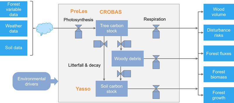
Fig. 2. The biochemical and biophysical modelling system PREBAS.
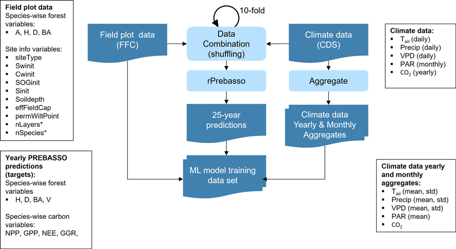
Fig. 3. Training data set construction. The forest variable and site info data from each FFC field plot were combined with the climate data (of random scenario, from random climate zone within 150 km distance from the filed plot’s forestry district border and covering random 25-year period within 2020–2100). The climate data randomized this way were joined 10 times for each field plot (10-fold shuffle). These combined data vectors were provided for rPrebasso as inputs to create the 25-year prediction targets. The climate data were aggregated to contain yearly and monthly averages and standard deviations. The data vector from each field plot were combined with the corresponding 25-year rPrebasso predictions, and aggregated climate data to construct the training data set for the ML models. FFC = Finnish Forest Centre, CDS = Climate Data Store. Forest variables: A = age, H = tree height, D = stem diameter, BA = basal area, V = stem volume; Site info variables: siteType = Site fertility class, Swinit = Initial soil water, Cwinit = Initial crown water, SOGinit = Initial snow on ground, Sinit = Initial temperature acclimation state, Soildepth = Soil depth, effFieldCap = Effective field capacity, permWiltPoint = Permanent wilting point, nLayers = Number of layers*, nSpecies = Number of species*; carbon balance variables: NPP = net primary production, GPP = gross primary production per tree layer, NEE = net ecosystem exchange, GGR = and gross growth; Climate variables: Tair = daily temperature, Precip = precipitation, VPD = vapour pressure deficit, PAR = monthly photosynthetically active radiation, CO2 = yearly CO2 concentration. Species-wise variables were used for the forest and carbon balance variables (e.g. Hpine, Hspr, Hbl; spr = spruce, bl = broadleaved).
*) The variables nLayers and nSpecies used by rPrebasso only, not provided for ML models.
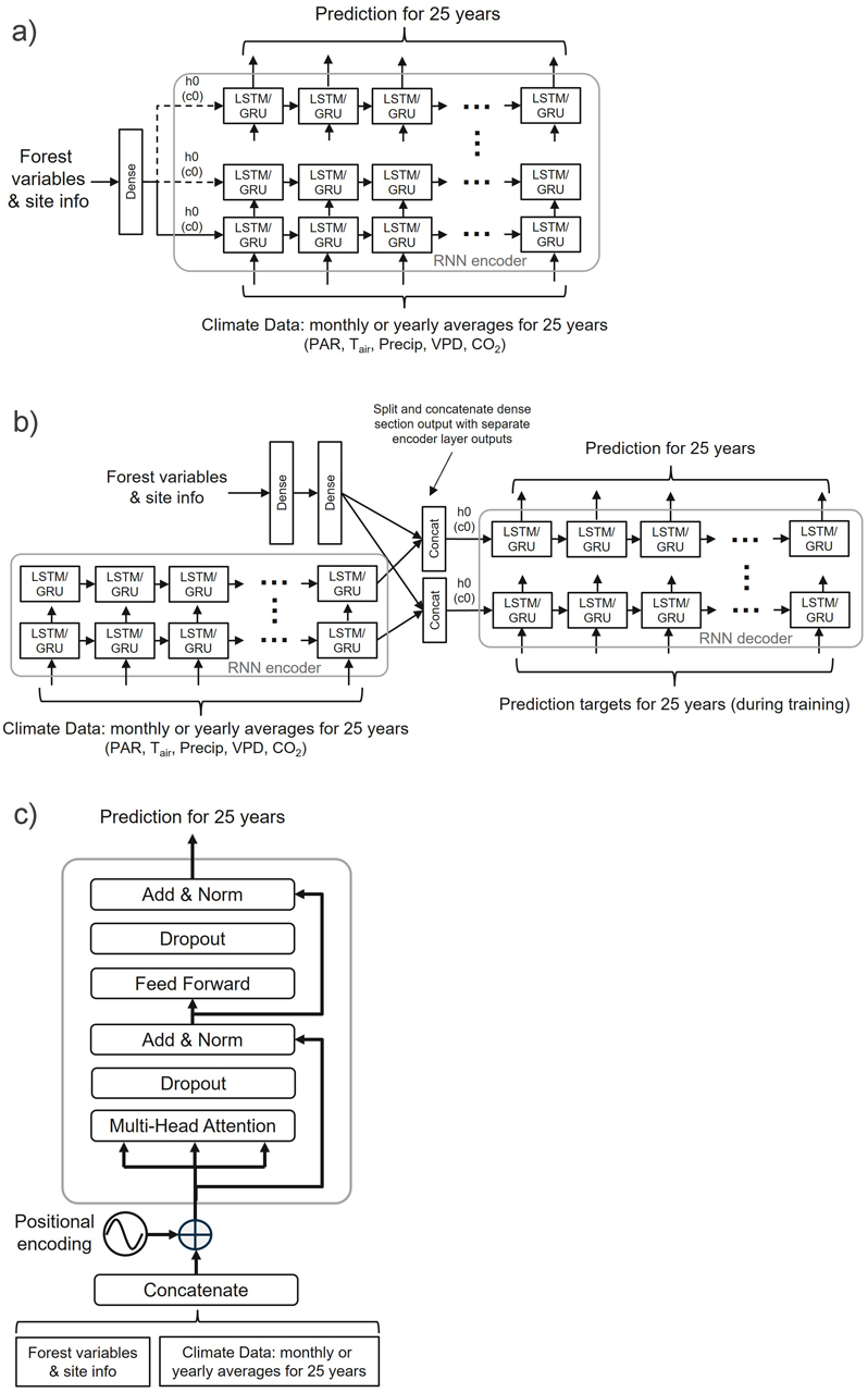
Fig. 4. General overview of the three neural network architectures used in the study: a) RNN encoder with a fully connected input section (FC-RNN), b) RNN encoder-decoder network combined with a fully connected section parallel to the encoder (S2S), and c) Transformer encoder network (TXFORMER). GRU = Gated Recurrent Unit, LSTM = Long short-term memory, PAR = photosynthetically active radiation, TAir = daily temperature, Precip = precipitation, VPD = vapour pressure deficit, CO2 = carbon dioxide, h0 = hidden state vector, c0 = cell state vector, N = number of decoder layers. The reader is suggested to visit the code repository for the detailed implementation of the models.
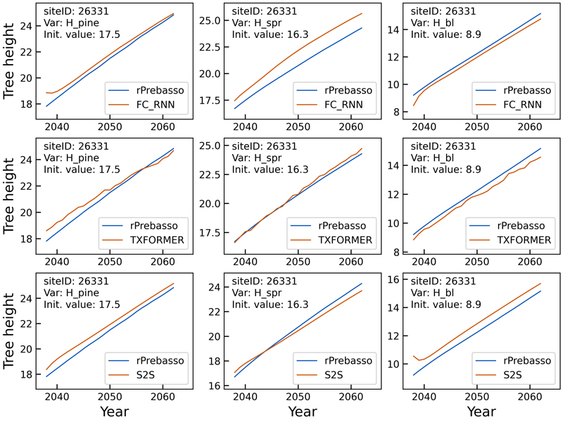
Fig. 5. Example of 25-year rPrebasso target and ML model prediction curves of tree height (Hpine, Hspr, Hbl) plotted for randomly selected test site (site-ID: 26331). Top row: FC-RNN model, middle row: TXFORMER model, bottom row: S2S model (the model shown in legend). The curves indicate relatively small differences between the models. The FC-RNN and S2S model curves progress more smoothly than the TXFORMER prediction in general. The difficulty of the FC-RNN model capturing the progression from the site initial state (year 0) to the first year(s) prediction is clearly visible with variables Hpine and Hbl. This can also be seen for the S2S model variable Hbl.
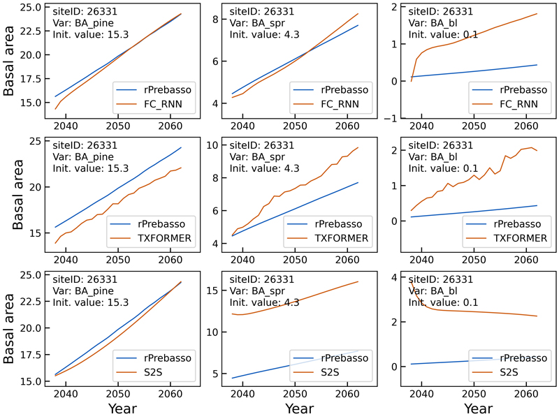
Fig. 6. Example of 25-year rPrebasso target and ML model prediction curves of basal area (BApine, BAspr, BAbl) plotted for randomly selected test site (site-ID: 26331). Top row: FC-RNN model, middle row: TXFORMER model, bottom row: S2S model (the model shown in legend). The differences between the model types are distinct. The FC-RNN model seems to best predict the BA progression, although the prediction for broadleaved species (BAbl) contains large offset.
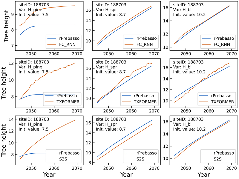
Fig. 7. Example of 25-year rPrebasso target and ML model prediction curves of tree height (Hpine, Hspr, Hbl) plotted for randomly selected test site (site-ID: 188703). Top row: FC-RNN model, middle row: TXFORMER model, bottom row: S2S model (the model shown in legend). The rPrebasso prediction of Hpine saturates after about nine years from the beginning of the prediction period. This behavior appeared to be difficult to capture by the ML models. The FC-RNN model performs best in replicating the rPrebasso curve, although with large offset. TXFORMER and S2S models fail to model the saturation. Note that 7.3% of the training data targets (rPrebasso predictions) showed this kind of saturation effect in tree height or stem diameter variables. The predictions for Hspr and Hbl are relatively good with all the models.
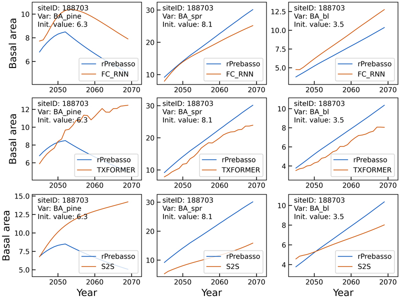
Fig. 8. Example of 25-year rPrebasso target and ML model prediction curves of basal area (BApine, BAspr, BAbl) plotted for randomly selected test site (site-ID: 188703). Top row: FC-RNN model, middle row: TXFORMER model, bottom row: S2S model (the model shown in legend). The decline in BApine target (rPrebasso prediction) after about nine years from the beginning of the prediction period could be captured by the FC-RNN model only, although with relatively large offset.
| Table 2. The mean, minimum and maximum of yearly (25 years) relative bias (BIAS%) and relative root mean squared errors (RMSE%) of the test set predictions computed for tree height (H), tree diameter (D), basal area (BA), and net primary production (NPP) for pine, spruce (spr) and broadleaved (bl) species. Results for model types: FC-RNN, TXFORMER, and S2S compared. LSTM RNN unit in FC_RNN and S2S models used. | |||||||||
| Model type | Variable | Relative bias (BIAS%) | Relative RMS error (RMSE%) | ||||||
| mean | mean* | min | max | mean | min | max | |||
| FC_RNN | Hpine | –0.1 | 0.3 | –0.6 | 0.4 | 6.8 | 6.1 | 8.3 | |
| FC_RNN | Hspr | –0.8 | 0.8 | –1.1 | –0.6 | 6.9 | 6.1 | 8.5 | |
| FC_RNN | Hbl | 0.4 | 0.4 | 0.3 | 0.5 | 5.5 | 5.2 | 6.2 | |
| TXFORMER | Hpine | 0.5 | 0.7 | –1.2 | 1.3 | 7.7 | 6.8 | 9.5 | |
| TXFORMER | Hspr | 0.7 | 0.7 | –0.4 | 1.3 | 8.0 | 6.9 | 10.1 | |
| TXFORMER | Hbl | 0.3 | 0.7 | –1.2 | 1.3 | 6.2 | 5.4 | 7.4 | |
| S2S | Hpine | –0.3 | 0.8 | –1.6 | 1.3 | 11.5 | 9.9 | 14.2 | |
| S2S | Hspr | –1.6 | 1.6 | –2.1 | –0.6 | 11.8 | 10.0 | 14.4 | |
| S2S | Hbl | 0.0 | 0.3 | –1.5 | 0.3 | 11.1 | 10.4 | 14.3 | |
| FC_RNN | Dpine | –0.6 | 0.6 | –0.9 | –0.3 | 6.5 | 5.6 | 8.1 | |
| FC_RNN | Dspr | –0.9 | 0.9 | –1.3 | –0.6 | 7.0 | 6.2 | 8.6 | |
| FC_RNN | Dbl | 0.1 | 0.1 | 0.0 | 0.7 | 6.9 | 6.5 | 8.2 | |
| TXFORMER | Dpine | 0.1 | 0.5 | –1.2 | 1.0 | 8.2 | 6.9 | 10.0 | |
| TXFORMER | Dspr | 0.2 | 0.5 | –1.2 | 0.9 | 10.3 | 9.9 | 11.5 | |
| TXFORMER | Dbl | –1.2 | 1.2 | –3.1 | 0.0 | 8.5 | 8.0 | 9.3 | |
| S2S | Dpine | –0.3 | 0.4 | –1.1 | 0.4 | 14.2 | 12.9 | 16.2 | |
| S2S | Dspr | –0.8 | 0.9 | –1.4 | 0.2 | 14.3 | 12.5 | 16.4 | |
| S2S | Dbl | 1.5 | 1.5 | 0.2 | 1.8 | 14.5 | 13.2 | 18.8 | |
| FC_RNN | BApine | –0.1 | 0.2 | –0.6 | 0.2 | 12.0 | 7.7 | 15.9 | |
| FC_RNN | BAspr | –1.5 | 1.5 | –1.8 | –0.8 | 15.6 | 11.9 | 19.2 | |
| FC_RNN | BAbl | 1.5 | 1.5 | 0.7 | 2.2 | 21.0 | 15.0 | 27.9 | |
| TXFORMER | BApine | –0.7 | 1.5 | –5.0 | 1.5 | 17.6 | 15.2 | 19.7 | |
| TXFORMER | BAspr | 0.8 | 1.0 | –1.4 | 1.8 | 22.1 | 16.4 | 26.5 | |
| TXFORMER | BAbl | –6.4 | 6.4 | –7.4 | –5.0 | 24.7 | 15.6 | 32.5 | |
| S2S | BApine | –0.8 | 1.9 | –3.1 | 3.2 | 45.5 | 41.0 | 54.7 | |
| S2S | BAspr | –10.5 | 10.7 | –17.4 | 2.0 | 63.8 | 61.7 | 67.9 | |
| S2S | BAbl | –21.0 | 21.2 | –34.9 | 2.0 | 86.0 | 82.5 | 99.1 | |
| FC_RNN | NPPpine | 1.2 | 1.3 | –0.1 | 2.4 | 11.6 | 9.9 | 15.5 | |
| FC_RNN | NPPspr | 0.8 | 0.8 | 0.5 | 1.1 | 14.8 | 13.5 | 20.4 | |
| FC_RNN | NPPbl | 1.9 | 1.9 | 0.4 | 3.2 | 22.0 | 20.2 | 28.2 | |
| TXFORMER | NPPpine | –0.7 | 0.9 | –3.6 | 0.7 | 19.9 | 18.5 | 23.6 | |
| TXFORMER | NPPspr | –0.2 | 0.9 | –3.1 | 1.0 | 27.8 | 26.9 | 31.3 | |
| TXFORMER | NPPbl | –2.8 | 2.8 | –4.5 | –1.7 | 30.9 | 28.8 | 32.2 | |
| S2S | NPPpine | 2.6 | 2.6 | –0.4 | 6.3 | 31.2 | 27.4 | 37.9 | |
| S2S | NPPspr | –4.6 | 7.0 | –10.4 | 9.5 | 44.3 | 37.3 | 51.4 | |
| S2S | NPPbl | –17.3 | 17.4 | –26.5 | 1.7 | 64.6 | 59.3 | 88.0 | |
| FC-RNN = recurrent neural network model with fully connected input section; TXFORMER = transformer model. S2S = RNN encoder-decoder model. RNN = Recurrent neural network; LSTM = Long short-term memory. *) The mean of absolute values of BIAS%. | |||||||||
| Table 3. The mean, minimum and maximum of yearly (25 years) relative bias (BIAS%) and relative root mean squared errors (RMSE%) of the test set predictions computed for gross primary production per tree layer (GPP), gross growth (GGR), and net ecosystem exchange (NEE) for pine, spruce (spr) and broadleaved (bl) species. GPP model: FC-RNN (GRU). GGR and NEE Models: FC-RNN (LSTM). | ||||||||
| Variable | Relative bias (BIAS%) | Relative RMS error (RMSE%) | ||||||
| mean | mean* | min | max | mean | min | max | ||
| GPPpine | 1.4 | 1.4 | 0.1 | 2.4 | 10.3 | 9.0 | 13.8 | |
| GPPspr | 0.6 | 0.6 | 0.4 | 0.9 | 11.8 | 10.9 | 16.7 | |
| GPPbl | 1.2 | 1.2 | 0.1 | 2.0 | 19.3 | 17.8 | 24.2 | |
| GGRpine | 1.9 | 1.9 | 0.5 | 2.5 | 19.4 | 17.4 | 24.5 | |
| GGRspr | –1.4 | 1.4 | –2.3 | –0.7 | 19.2 | 18.1 | 23.3 | |
| GGRbl | 0.2 | 0.6 | –0.6 | 1.6 | 28.0 | 25.4 | 31.3 | |
| NEEpine | 0.8 | 0.8 | 0.4 | 1.7 | 13.2 | 11.0 | 17.4 | |
| NEEspr | 1.3 | 1.3 | 0.5 | 1.9 | 17.4 | 15.8 | 20.6 | |
| NEEbl | 0.4 | 0.4 | –0.2 | 1.4 | 25.4 | 23.7 | 27.3 | |
| FC-RNN = recurrent neural network model with fully connected input section; RNN = Recurrent neural network; LSTM = Long short-term memory; GRU = Gated recurrent unit. *) The mean of absolute values of BIAS%. | ||||||||
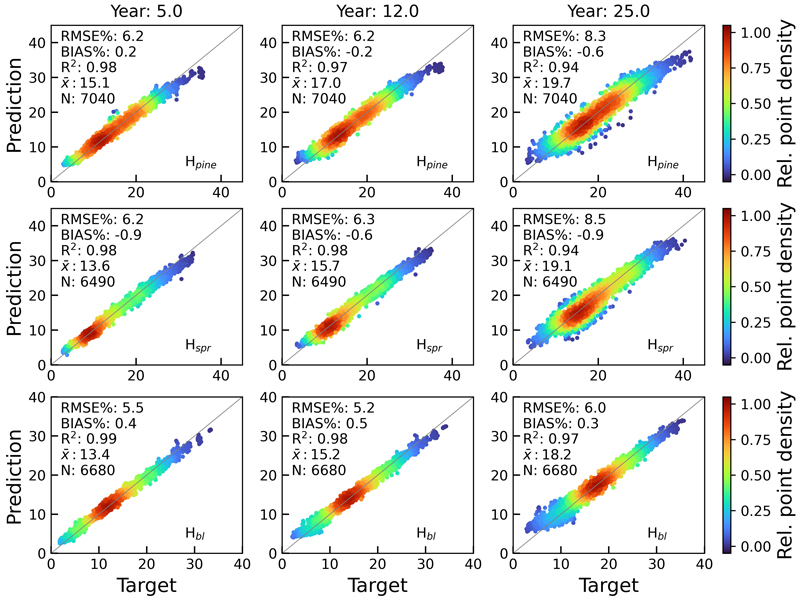
Fig. 9. Scatterplots of test set tree height predictions for pine (Hpine), spruce (Hspr) and broadleaved (Hbl) species against rPrebasso estimates (target) for years 5, 12 and 25. Model = FC-RNN (LSTM). RMSE% = relative RMS-error, BIAS% = relative bias, R2 = coefficient of determination, ![]() = the average of the target values, N = number of samples. The colour shows the relative density of the graph points. FC-RNN = RNN encoder model with a fully connected input section; LSTM = Long short-term memory. RNN = Recurrent neural network.
= the average of the target values, N = number of samples. The colour shows the relative density of the graph points. FC-RNN = RNN encoder model with a fully connected input section; LSTM = Long short-term memory. RNN = Recurrent neural network.
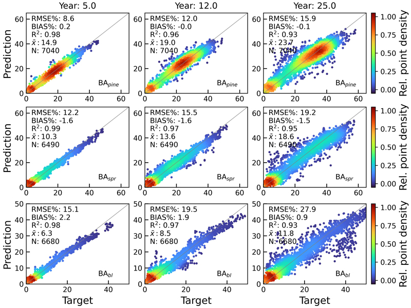
Fig. 10. Scatterplots of test set basal area predictions for pine (BApine), spruce (BAspr) and broadleaved (BAbl) species against rPrebasso estimates (target) for years 5, 12 and 25. Model = FC-RNN (LSTM). RMSE% = relative RMS-error, BIAS% = relative bias, R2 = coefficient of determination, ![]() = the average of the target values, N = number of samples. The colour shows the relative density of the graph points. FC-RNN = RNN encoder model with a fully connected input section; LSTM = Long short-term memory. RNN = Recurrent neural network.
= the average of the target values, N = number of samples. The colour shows the relative density of the graph points. FC-RNN = RNN encoder model with a fully connected input section; LSTM = Long short-term memory. RNN = Recurrent neural network.
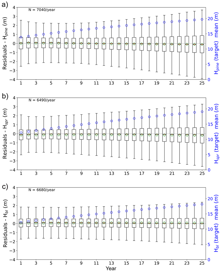
Fig. 11. Boxplots of test set yearly residual errors for the tree height of a) pine (Hpine), b) spruce (Hspr) and c) broadleaved (Hbl) species. Model: FC-RNN (LSTM). Green diamond = mean, red line = median. Right hand scale: the yearly mean of the target variable (plotted with blue circles). FC-RNN = RNN encoder model with a fully connected input section; LSTM = Long short-term memory. RNN = Recurrent neural network.
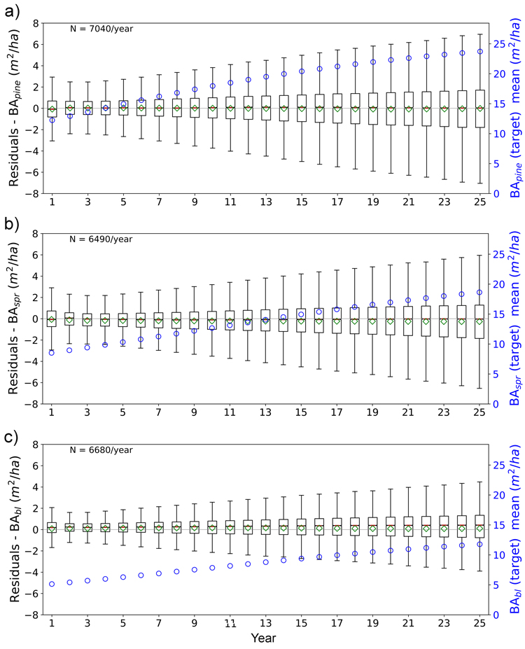
Fig. 12. Boxplots of test set yearly residual errors for the basal area of a) pine (BApine), b) spruce (BAspr) and c) broadleaved (BAbl) species. Model: FC-RNN (LSTM). Green diamond = mean, red line = median. Right hand scale: the yearly mean of the target variable (plotted with blue circles). FC-RNN = RNN encoder model with a fully connected input section; LSTM = Long short-term memory. RNN = Recurrent neural network.
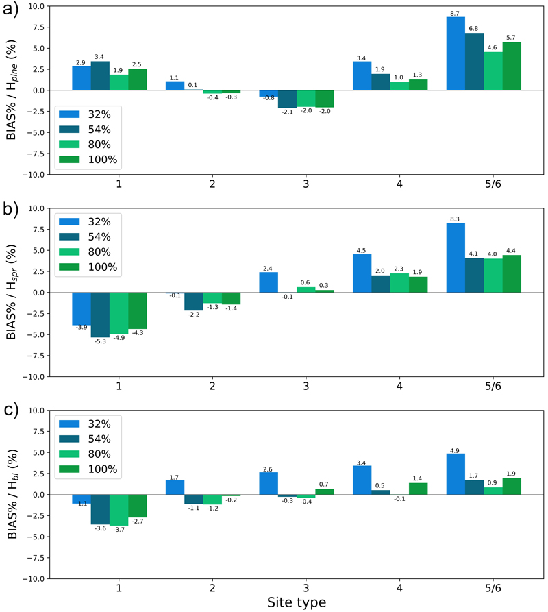
Fig. 13. The test set relative bias (BIAS%) for year 25 plotted per site type for the tree height of a) pine (Hpine), b) spruce (Hspr) and c) broadleaved (Hbl) species. The bars of different colours represent models trained with 32%, 54%, 80% or 100% of the training data set. The fertility classes 5 and 6 were treated as a single class by rPrebasso. Model FC-RNN (LSTM). FC-RNN = RNN encoder model with a fully connected input section; LSTM = Long short-term memory. RNN = Recurrent neural network.
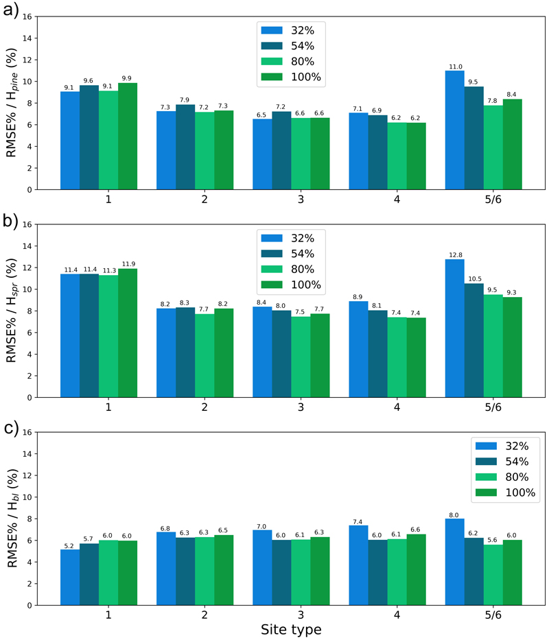
Fig. 14. The test set relative RMS error (RMSE%) for year 25 plotted per site type for the tree height of a) pine (Hpine), b) spruce (Hspr) and c) broadleaved (Hbl) species. The bars of different colours represent models trained with 32%, 54%, 80% or 100% of the training data set. The fertility classes 5 and 6 were treated as a single class by rPrebasso. Model FC-RNN (LSTM). FC-RNN = RNN encoder model with a fully connected input section; LSTM = Long short-term memory. RNN = Recurrent neural network.
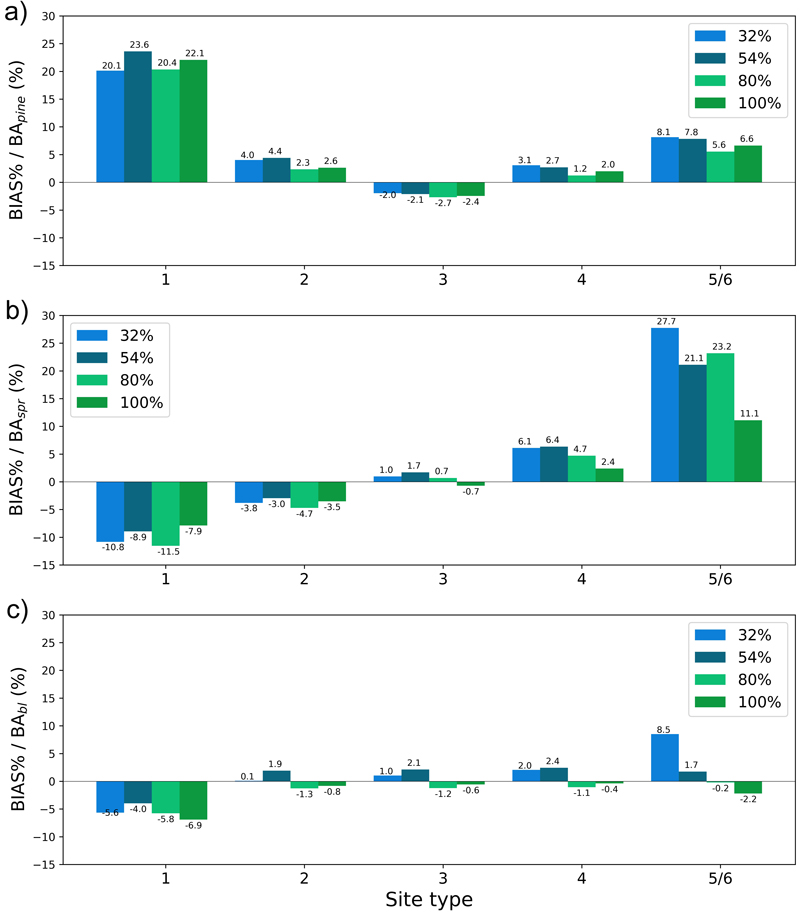
Fig. 15. The test set relative bias (BIAS%) for year 25 plotted per site type category for the basal area of a) pine (BApine), b) spruce (BAspr) and c) broadleaved (BAbl) species. The bars of different colours represent models trained with 32%, 54%, 80% or 100% of the training data set. The fertility classes 5 and 6 were treated as a single class by rPrebasso. Model FC-RNN (LSTM). FC-RNN = RNN encoder model with a fully connected input section; LSTM = Long short-term memory. RNN = Recurrent neural network.
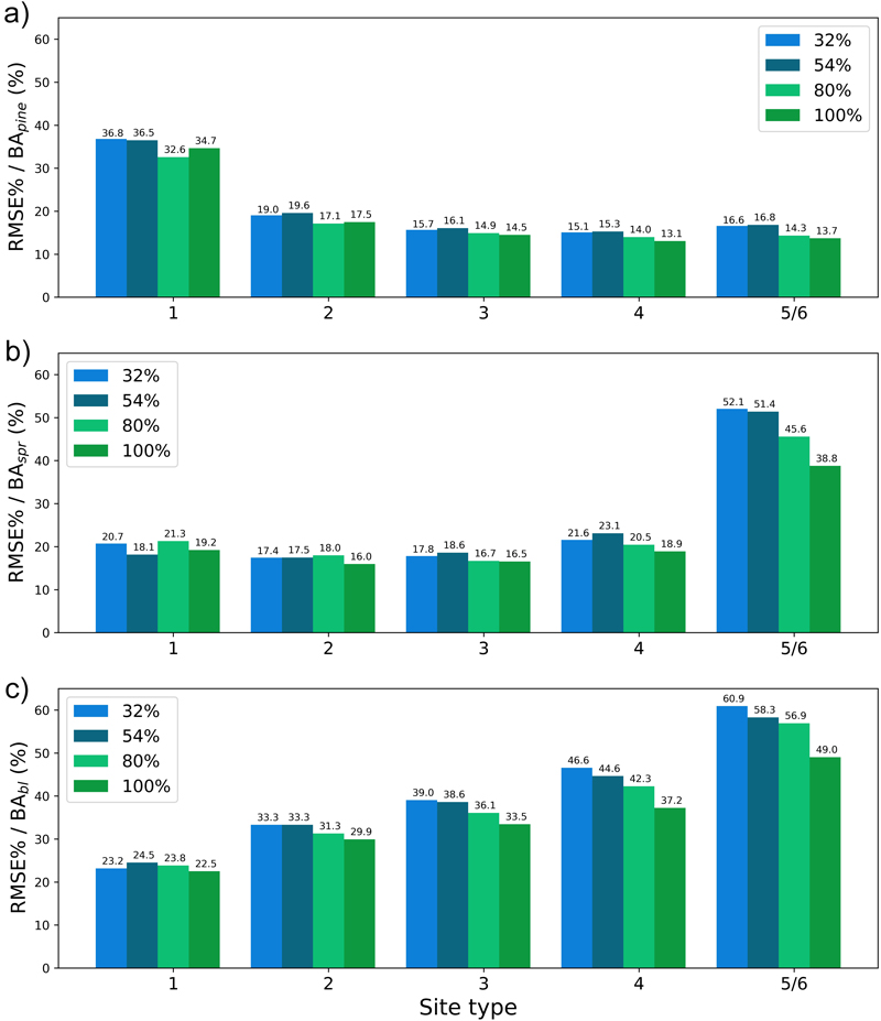
Fig. 16. The test set relative RMS error (RMSE%) for year 25 plotted per site type category for the basal area of a) pine (BApine), b) spruce (BAspr) and c) broadleaved (BAbl) species. The bars of different colours represent models trained with 32%, 54%, 80% or 100% of the training data set. The fertility classes 5 and 6 were treated as a single class by rPrebasso. Model FC-RNN (LSTM). FC-RNN = RNN encoder model with a fully connected input section; LSTM = Long short-term memory. RNN = Recurrent neural network.
| Table 4. The mean, minimum, maximum, and standard deviation of the correlation between the species-wise tree height (H) and stem diameter (D) predictions of test data set. The results of rPrebasso predictions indicated by the suffix ‘PR’, and the results of the machine learning models by the suffix ‘ML’. Results of the three model types FC-RNN (LSTM), TXFORMER, and S2S (LSTM) compared. | ||||||||||
| Model | Species | mean_PR | min_PR | max_PR | std_PR | mean_ML | min_ML | max_ML | std_ML | N |
| FC_RNN | pine | 0.999 | 0.993 | 1.000 | 0.001 | 0.993 | –0.013 | 1.000 | 0.032 | 7040 |
| FC_RNN | spr | 0.989 | –1.000 | 1.000 | 0.127 | 0.994 | –0.696 | 1.000 | 0.049 | 6490 |
| FC_RNN | bl | 0.999 | 0.400 | 1.000 | 0.015 | 0.995 | –0.407 | 1.000 | 0.027 | 6680 |
| TXFORMER | pine | 0.999 | 0.993 | 1.000 | 0.001 | 0.996 | 0.565 | 1.000 | 0.017 | 7040 |
| TXFORMER | spr | 0.989 | –1.000 | 1.000 | 0.127 | 0.997 | 0.901 | 1.000 | 0.004 | 6490 |
| TXFORMER | bl | 0.999 | 0.400 | 1.000 | 0.015 | 0.997 | 0.440 | 1.000 | 0.014 | 6680 |
| S2S | pine | 0.999 | 0.993 | 1.000 | 0.001 | 0.996 | 0.889 | 1.000 | 0.005 | 7040 |
| S2S | spr | 0.989 | –1.000 | 1.000 | 0.127 | 0.997 | 0.959 | 1.000 | 0.003 | 6490 |
| S2S | bl | 0.999 | 0.400 | 1.000 | 0.015 | 0.994 | 0.585 | 1.000 | 0.029 | 6680 |