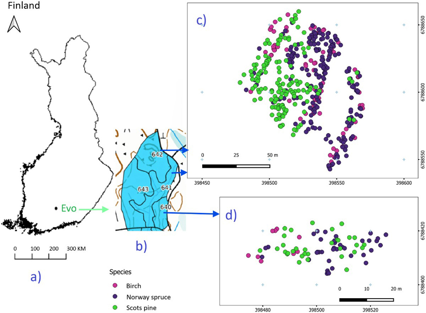
Fig. 1. Study area (a) and forest stands (b), with harvested tree species from the northern (c) and southern (d) parts.
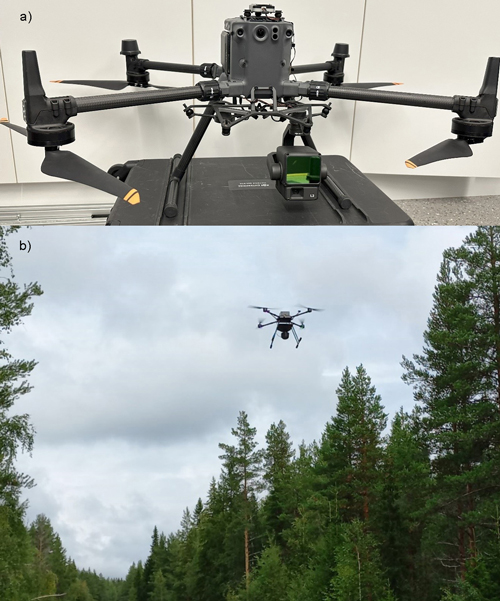
Fig. 2. Drone-based laser scanning (DLS) setup and forest scanning: Zenmuse L2 laser scanner with DJI Matrice 350 RTK drone (a), and forest scanning with DLS (b).
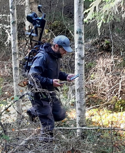
Fig. 3. Forest scanning with backpack Faro Orbis mobile laser scanner.
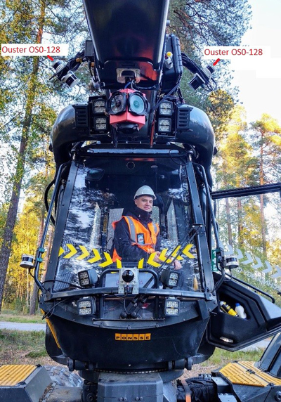
Fig. 4. Two Ouster OS0-128 LiDARs set up on Ponsse Scorpion harvester.
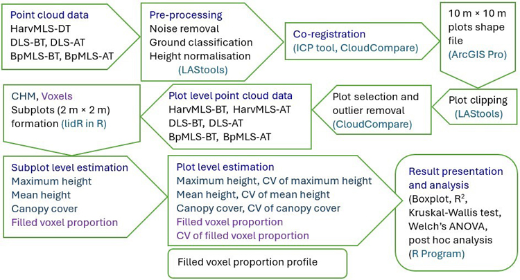
Fig. 5. Workflow of this study. The process begins with the acquisition of point cloud data and proceeds through pre-processing, processing, and analysis stages. Point cloud data were collected using harvester-mounted mobile laser scanning (HarvMLS), backpack mobile laser scanning (BpMLS), and drone-based laser scanning (DLS). HarvMLS data were obtained during thinning (DT), while DLS and BpMLS data were collected both before thinning (BT) and after thinning (AT). The study adopted open-source tools and packages, including LAStools, Cloudcompare, ArcGIS Pro, lidR, and R Studio.
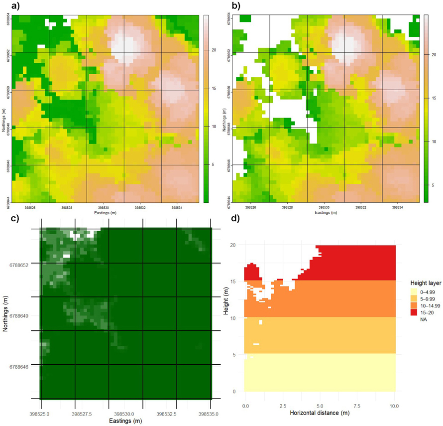
Fig. 6. Division of a sample plot (10 m × 10 m) into subplots and vertical strata to quantify forest structure. The plot was subdivided into 2 m × 2 m subplots, and canopy height models (CHMs) were generated within each subplot to estimate height (a) and cover attributes (b). Top-down view showing filled voxel proportion at the subplot scale (c). Filled voxel proportion at different height levels were computed using a voxel size of 20 cm (d). Subplot-level values were further used to calculate mean values and coefficients of variation (CVs). View larger in new window/tab.
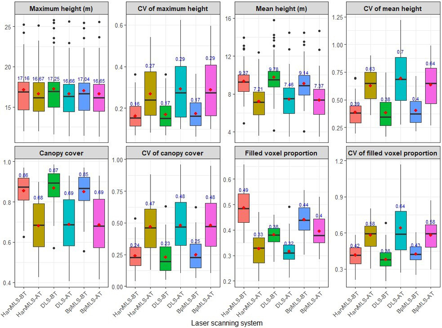
Fig. 7. Forest structural attributes quantified before and after thinning using three laser scanning systems. The assessed attributes included maximum height, mean height, canopy cover, and filled voxel proportion, with the coefficient of variation (CV) calculated for each attribute. Data were obtained from a harvester-mounted mobile laser scanner (HarvMLS), a drone-based laser scanner (DLS) and a backpack mobile laser scanner (BpMLS). Conditions are shown before thinning (BT) and after thinning (AT), with mean values indicated in red.
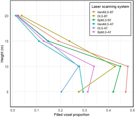
Fig. 8. Filled voxel proportion values across the different heights. Data were obtained from a harvester-mounted mobile laser scanner (HarvMLS), a backpack mobile laser scanner (BpMLS) and a drone-based laser scanner (DLS). Conditions are shown before thinning (BT) and after thinning (AT).
| Table 1. Results of Kruskal–Wallis test and Welch’s ANOVA for forest structural attributes derived from harvester-mounted mobile laser scanner (HarvMLS), backpack mobile laser scanner (BpMLS) and drone-based laser scanner (DLS). Chi-square value (χ2) and F value are reported for the Kruskal–Wallis test (K–W) and Welch’s ANOVA (W) test, respectively. CV denotes coefficient of variation. Significant p-values are indicated in bold. | ||||||
| Forest structural attribute | Test value | p-value | Adjusted p-value | Statistical analysis | ||
| HarvMLS vs DLS | BpMLS vs DLS | BpMLS vs HarvMLS | ||||
| Maximum height | 0.423 | 0.809 | 1.00 | 0.889 | 0.834 | K–W |
| CV maximum height | 0.592 | 0.743 | 0.939 | 1.00 | 0.670 | K–W |
| Mean height | 2.053 | 0.358 | 0.435 | 0.257 | 1.00 | K–W |
| CV mean height | 0.068 | 0.966 | 1.00 | 1.00 | 1.00 | K–W |
| Canopy cover (CC) | 0.914 | 0.633 | 0.561 | 0.679 | 1.00 | K–W |
| CV of CC | 0.210 | 0.899 | 1.00 | 0.971 | 1.00 | K–W |
| Filled voxel proportion (FVP) | 51.224 | <0.001 | <0.001 | <0.001 | 0.103 | K–W |
| CV of FVP | 2.398 | 0.301 | 0.272 | 0.267 | 1.00 | K–W |
| FVP profile | ||||||
| <5 m | 115.58 | < 0.001 | <0.001 | <0.001 | 0.483 | (W) test |
| 5–9.99 m | 9.004 | 0.011 | 0.129 | 0.004 | 0.303 | K–W |
| 10–14.99 m | 23.11 | <0.001 | <0.001 | <0.001 | 0.565 | K–W |
| 15–20 m | 1.377 | 0.502 | 1.00 | 0.431 | 0.503 | K–W |