| Table 1. Information on the sample plots. Remaining stand basal area (Gafter) in moderate (less intensive) and heavy (intensive) cutting was 17 and 12–13 m2 ha–1, respectively. Gbefore = stand basal area before cutting. n = number of sample plots. Drained peatland forest type (Laine et al. 2018), Rhtkg (I) and (II) = herb-rich types (I) and (II), Mtkg(I) = Vaccinium myrtillus type (I), Mtkg(I-) = more infertile border variant of Mtkg(I). | |||||
| Municipality | Treatment | Gafter | Gbefore | n | Site type |
| Heinävesi (Rouvanlehto) | Control | 22–23 | 22–23 | 2 | Rhtkg(I) |
| Moderate | 17 | 21–24 | 2 | Rhtkg(I) | |
| Heavy | 12 | 22 | 2 | Rhtkg(I) | |
| Janakkala (Paroninkorpi) | Control | 22–30 | 22–30 | 5 | Rhtkg(II) |
| Moderate | 17 | 22–27 | 5 | Rhtkg(II) | |
| Heavy | 12 | 23–31 | 5 | Rhtkg(II) | |
| Juuka (Vaarajoki) | Control | 20–22 | 20–22 | 2 | Mtkg(I) |
| Moderate | 17 | 19–24 | 2 | Mtkg(I) | |
| Heavy | 12 | 25–29 | 2 | Mtkg(I) | |
| Multia (Havusuo) | Control | 25–28 | 25–28 | 2 | Mtkg(I) – Mtkg(I-) |
| Heavy | 13 | 29–31 | 2 | Mtkg(I) – (Mtkg(I-) | |
| Table 2. Two-way repeated measures ANOVA with treatment (thinning intensity) and year (time since harvest) as fixed factors on the percent cover of species groups and species in the cutting trials on drained peatlands (Eq. 1). F-values and corresponding p-values indicated by asterisks (* p < 0.05, ** p < 0.01, *** p < 0.001) are presented only for the species groups and species with significant (p < 0.05) effects. For species abbreviations, see the text and Supplementary file S1. | ||||
| Species groups or species | Intercept | Treatment | Year | Treatment × Year |
| TREES and SHRUBS | 69.58** | 2.34 | 8.41*** | 3.20* |
| DWARF SHRUBS | 486.22*** | 0.29 | 37.33*** | 8.01*** |
| GRASSES and SEDGES | 10.66* | 4.12* | 34.13*** | 9.14*** |
| HERBS | 75.47** | 0.17 | 15.10*** | 5.51*** |
| BRYALES | 809.24*** | 1.72 | 17.20*** | 3.17* |
| SPHAGNUM | 302.12*** | 0.78 | 11.22*** | 1.21 |
| Betupube | 28.54* | 3.73* | 4.88* | 4.04** |
| Piceabie | 26.18* | 0.15 | 3.40* | 1.12 |
| Pinusylv | 7.43* | 2.32 | 5.85** | 1.84 |
| Rubuidae | 25.76* | 4.50* | 19.68*** | 5.80*** |
| Sorbaucu | 7.96 | 0.83 | 6.53** | 0.50 |
| Vaccmyrt | 82.98** | 0.15 | 49.48*** | 5.44** |
| Vaccviti | 36.19** | 1.14 | 9.01*** | 7.00*** |
| Careglob | 7.28 | 2.41 | 23.55*** | 6.40*** |
| Descflex | 5.37 | 0.84 | 6.08** | 1.02 |
| Dryocart | 185.00*** | 0.41 | 35.25*** | 2.73* |
| Epilangu | 15.31*** | 1.47 | 6.78** | 3.55* |
| Linnbore | 4.15 | 0.25 | 3.39* | 2.86* |
| Maiabifo | 3.45 | 0.33 | 7.61** | 0.46 |
| Melasylv | 1.85 | 2.37 | 3.05 | 2.85* |
| Oxalacet | 2.84 | 1.57 | 5.60** | 4.00** |
| Trieeuro | 10.76* | 4.50* | 17.10*** | 3.62* |
| Bracspp | 41.30* | 1.02 | 7.72** | 7.46*** |
| Dicrmaju | 26.18* | 2.94 | 26.32*** | 0.57 |
| Hylosple | 255.26*** | 0.39 | 14.82*** | 3.24* |
| Plagspp | 2.20 | 0.39 | 9.23*** | 1.46 |
| Pleuschr | 53.11** | 0.55 | 11.63*** | 3.63* |
| Sphagirg | 12.17* | 0.42 | 6.57** | 1.86 |
| Spharuss | 6.70 | 0.39 | 7.55** | 0.23 |
| Litter | 1088.50*** | 0.87 | 22.30*** | 2.85* |
| Number of species | 690.35*** | 0.42 | 4.17* | 2.95* |
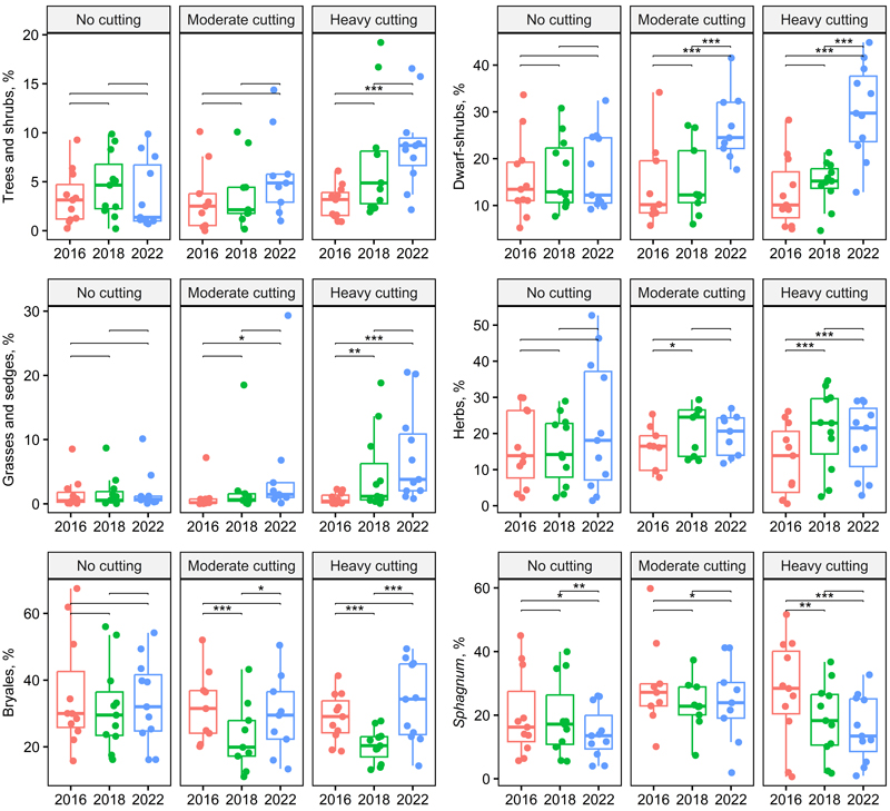
Fig. 1. Box plots showing species group cover across treatment and year (two-way repeated ANOVA, Table 2). Significant pairwise comparisons among years are indicated with asterisks (* p < 0.05, ** p < 0.01, *** p < 0.001). Treatments and stand basal area after cutting in 2016: no cutting (G = 20–30 m2 ha–1), moderate cutting (G = 17 m2 ha–1) and heavy cutting (G = 12–13 m2 ha–1).

Fig. 2. Box plots showing the tree and shrub species cover across treatment and year (two-way repeated ANOVA, Table 2). Significant pairwise comparisons among years are indicated with asterisks (* p < 0.05, ** p < 0.01, *** p < 0.001). Treatments and stand basal area after cutting in 2016: no cutting (G = 20–30 m2 ha–1), moderate cutting (G = 17 m2 ha–1) and heavy cutting (G = 12–13 m2 ha–1).
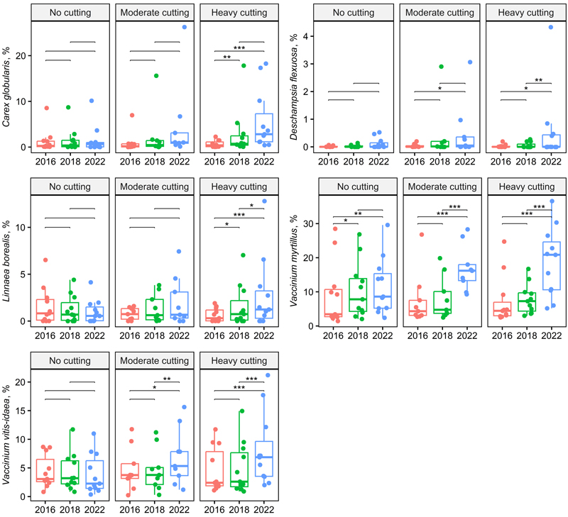
Fig. 3. Box plots showing grass and sedge and dwarf shrub species cover across treatment and year (two-way repeated ANOVA, Table 2). Significant pairwise comparisons among years are indicated with asterisks (* p < 0.05, ** p < 0.01, *** p < 0.001). Treatments and stand basal area after cutting in 2016: no cutting (G = 20–30 m2 ha–1), moderate cutting (G = 17 m2 ha–1) and heavy cutting (G = 12–13 m2 ha–1).
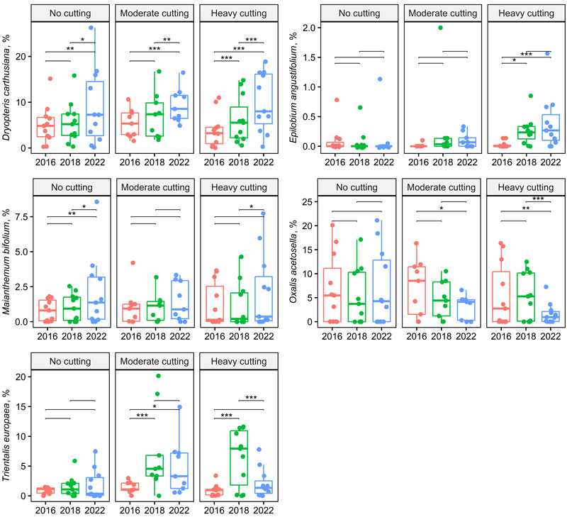
Fig. 4. Box plots showing herb species cover across treatment and year (two-way repeated ANOVA, Table 2). Significant pairwise comparisons among years are indicated with asterisks (* p < 0.05, ** p < 0.01, *** p < 0.001). Treatments and stand basal area after cutting in 2016: no cutting (G = 20–30 m2 ha–1), moderate cutting (G = 17 m2 ha–1) and heavy cutting (G = 12–13 m2 ha–1).
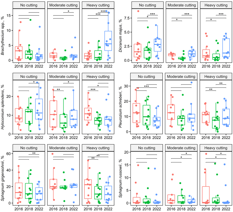
Fig. 5. Box plots showing the bryales and Sphagnum species cover across treatment and year (two-way repeated ANOVA, Table 2). Significant pairwise comparisons among years are indicated with asterisks (* p < 0.05, ** p < 0.01, *** p < 0.001). Treatments and stand basal area after cutting in 2016: no cutting (G = 20–30 m2 ha–1), moderate cutting (G = 17 m2 ha–1) and heavy cutting (G = 12–13 m2 ha–1).