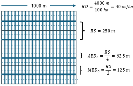
Fig. 1. Theoretical illustration of an ideal case of forest area of 100 ha, with 4 straight forest roads, mean road spacing (RS) of 250 m, road density (RD) of 40 m ha–1, calculative average extraction distance (AED0) of 62.5 m and calculative maximum extraction distance (MED0) of 125 m.
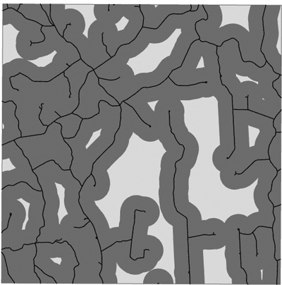
Fig. 2. A forest area of 2456 ha from Central Finland having forest roads of 62 406 m (25.4 m ha–1). With MED0 of 200 m (~RS/2), the accessibility index E = 0.708. The black vector line describes road network and dark grey the 200 m buffer around the road lines. Light grey describes the forest area that cannot be accessed with the MED0 of 200 m from the closest road.
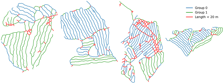
Fig. 3. Illustration of grouping of segments. Small line segments (<20 m) are removed (red-coloured segments). Remaining line segments are grouped based on their orientation using the K-means algorithm (blue and green coloured segments).
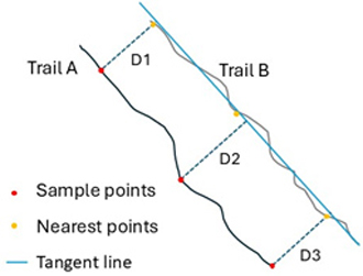
Fig. 4. Illustration of the distance calculation between adjacent trails.
| Table 1. Summary of the logging trail network metrics. | |||
| Definition | Equation | ||
| Metrics that analyse quantitative aspects of the logging trail network | TL | Logging trail network length (m), derived from the logging trail network polyline | |
| Atot | Area (m2) of the logging site polygon | ||
| TD | Logging trail network density (m ha–1) | ||
| TSn | Nominal logging trail spacing (m) | ||
| DIST | Distance travelled (m), calculated as the sum of segment lengths multiplied by the number of machine passes | ||
| Quantitative metrics considering buffer polygon regions | AT | Logging trail area (m2), calculated as TL multiplied by the nominal trail width (e.g., 4.5 m) | |
| AT% | Proportion of trail area within the logging site (%), calculated as AT/Atot | ||
| ANBRC | Net boom reach coverage (m2), defined as the total area reachable within the nominal crane length (~10 m). Areas extending beyond the logging site polygon are clipped | ||
| ATSC | Net coverage (m2) reached with the nominal logging trail spacing (TSn) | ||
| Spatial configuration metrics of the logging trail network | CA | Measures the share of the forest area that is reachable by the modern harvester | |
| TD0 | The density of the ideal logging trail network | ||
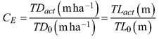
| CE | Compares the actual trail length, TLact, to the ideal trail length, TL0, or actual trail length density, TDact, to the ideal trail length density, TD0 | ||
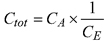
| Ctot | Structural-Coverage Efficiency index. Combines coefficients CA and CE | ||
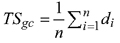
| TSgc | Average logging trail spacing | ||


| Table 2. Estimation of GNSS tracks per logging trail segment and the parameter values employed to consolidate the centerline (based on the algorithms by Cao et al. 2025). | ||||||
| Stand | No. of tracks per logging trail segment | Origin of GNSS Tracks H = harvester H+F = harvester and forwarder | Kernel density search radius | Threshold value | ||
| No. | Min | Max | Most frequent | |||
| 1 | 1 | 5 | 2 | H | 1.5 | 0.70 |
| 2 | 1 | 14 | 4 | H+F | 1.5 | 0.70 |
| 3 | 1 | 14 | 14 | H+F | 0.65 | 0.85 |
| 4 | 1 | 14 | 2 | H+F | 1.5 | 0.70 |
| 5 | 1 | 5 | 2 | H | 2.5 | 0.80 |
| 6 | 1 | 5 | 2 | H | 1.5 | 0.70 |
| 7 | 1 | 14 | 6–7 | H+F | 2 | 0.80 |
| 8 | 1 | 8–9 | 2 | H+F | 2.5 | 0.80 |
| 9 | 1 | 14 | 6–7 | H+F | 1.5 | 0.70 |
| 10 | 1 | 14 | 4 | H+F | 1.5 | 0.70 |
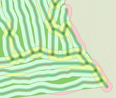
Fig. 5. Part of logging site 1. The site polygon is shown in dark green, the 10 m buffer around the logging trails in light green, and the logging trail area in medium green. Yellow areas indicate overlaps of the boom reach, while red areas represent boom reach extending outside the stand polygon.
| Table 3. Summary of logging trail network metric values by sample stand. | |||||||||
| Stand No. | Stand area Atot ha | Trail length TL m | Trail density TD m ha–1 | Trail spacing TSgc m | Share of trail area AT% | Net boom reach coverage ANBRC m2 | Coverage Coefficient CA | Structural Efficiency CE | Structural – Coverage Efficiency index Ctot = CA × CE–1 |
| 1 | 13.4 | 6558 | 487 | 20.0 | 21.4 | 10.9 | 0.81 | 0.98 | 0.83 |
| 2 | 19.8 | 9561 | 482 | 20.8 | 21.4 | 16.6 | 0.84 | 0.97 | 0.87 |
| 3 | 10.5 | 6244 | 594 | 20.3 | 25.7 | 19.0 | 0.87 | 1.19 | 0.73 |
| 4 | 13.9 | 9077 | 652 | 16.9 | 27.8 | 11.8 | 0.85 | 1.30 | 0.65 |
| 5 | 26.6 | 14292 | 537 | 21.4 | 23.7 | 23.2 | 0.87 | 1.07 | 0.81 |
| 6 | 7.83 | 4220 | 538 | 23.0 | 23.9 | 6.89 | 0.88 | 1.08 | 0.81 |
| 7 | 1.68 | 950 | 566 | 20.0 | 24.9 | 1.54 | 0.92 | 1.13 | 0.81 |
| 8 | 4.62 | 2526 | 546 | 20.0 | 23.9 | 3.92 | 0.85 | 1.09 | 0.78 |
| 9 | 6.29 | 3801 | 604 | 19.4 | 26.6 | 5.74 | 0.91 | 1.21 | 0.75 |
| 10 | 13.1 | 6590 | 502 | 23.4 | 22.2 | 11.3 | 0.86 | 1.0 | 0.86 |
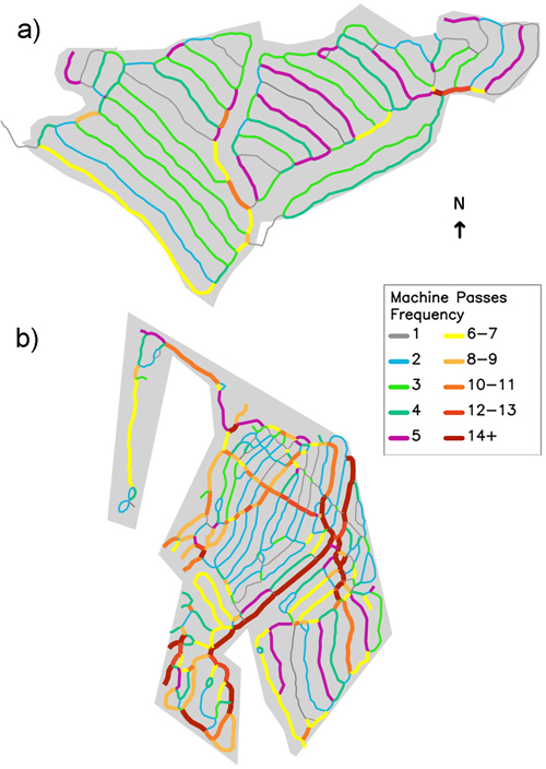
Fig. 6. Logging trail network of stand 10 (a), demonstrating a well-designed layout, and of stand 4 (b), demonstrating a poorly executed layout. Color-coding represents the number of machine passes.
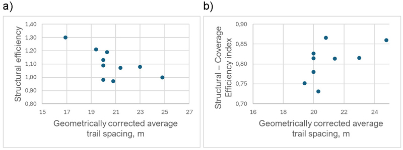
Fig. 7. In our small sample of ten sites, the geometrically corrected trail spacing (TSgc) was moderately correlated with the Structural Efficiency (r = –0.664, p = 0.036) (a) and with the Structural-Coverage Efficiency index (r = 0.753, p = 0.012) (b).