| Table 1. General information for 12 Salix viminalis populations across two basins in China. | |||||
| Population | River | Basin | Latitude, Longitude | Altitude (m a.s.l.) | Samples |
| MDG1 | Mordaga upstream | Ergun | 51°16´N, 120°44´E | 673 | 30 |
| MDG2 | Mordaga downstream | Ergun | 51°25´N, 120°00´E | 572 | 30 |
| GH | Genhe | Ergun | 50°46´N, 121°30´E | 706 | 30 |
| TL | Tuli | Ergun | 50°29´N, 121°41´E | 734 | 28 |
| KDE | Kuduer | Ergun | 50°02´N, 121°40´E | 848 | 27 |
| ZD1 | Zhadun | Ergun | 49°20´N, 120°40´E | 649 | 30 |
| ZD2 | Zhadun | Ergun | 49°20´N, 120°41´E | 650 | 30 |
| ZD3 | Zhadun | Ergun | 49°19´N, 120°40´E | 650 | 30 |
| YM | Yimin tributary | Ergun | 48°42´N, 119°47´E | 662 | 18 |
| HH | Huihe | Ergun | 48°04´N, 119°38´E | 772 | 17 |
| DHQ | Dahaiqing | West Liao | 44°14´N, 118°20´E | 1162 | 30 |
| HL | Heili | West Liao | 41°21´N, 118°27´E | 1049 | 30 |
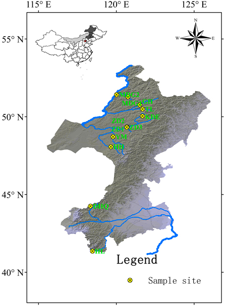
Fig. 1. Geographic locations of 12 Salix viminalis populations across two basins in China. [Note: Abbreviations of populations are explained in Table 1].
| Table 2. Genetic diversity of 12 populations in Salix viminalis based on 20 SSR markers. | ||||||
| Population | Na | Ne | Ho | He | FIS | Np |
| MDG1 | 8.600 | 4.701 | 0.671 | 0.737 | 0.073 | 3 |
| MDG2 | 9.150 | 4.743 | 0.637 | 0.719 | 0.098 | 8 |
| GH | 9.600 | 5.176 | 0.657 | 0.734 | 0.083 | 6 |
| TL | 10.50 | 5.524 | 0.650 | 0.754 | 0.120 | 14 |
| KDE | 9.100 | 5.549 | 0.728 | 0.757 | 0.020 | 7 |
| ZD1 | 9.200 | 4.275 | 0.667 | 0.705 | 0.037 | 8 |
| ZD2 | 8.950 | 4.596 | 0.650 | 0.726 | 0.079 | 0 |
| ZD3 | 9.400 | 4.709 | 0.655 | 0.748 | 0.104 | 4 |
| YM | 8.200 | 4.220 | 0.658 | 0.712 | 0.043 | 2 |
| HH | 7.050 | 4.143 | 0.653 | 0.718 | 0.072 | 1 |
| DHQ | 6.150 | 2.825 | 0.542 | 0.587 | 0.064 | 1 |
| HL | 3.850 | 2.187 | 0.490 | 0.473 | –0.059 | 2 |
| Mean | 8.313 | 4.387 | 0.638 | 0.698 | 0.062 | 4.670 |
| Abbreviations of populations are explained in Table 1. Na = Number of observed alleles; Ne = Number of effective alleles; Ho = Observed heterozygosity; He = Expected heterozygosity; FIS = Inbreeding coefficient among individuals within subpopulation; Np = Number of private alleles. | ||||||
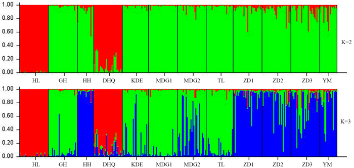
Fig. 2. Estimated population structure of 330 individuals in Salix viminalis with K = 2 and 3. [Note: Abbreviations of populations are explained in Table 1].
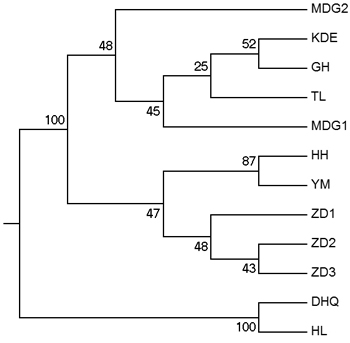
Fig. 3. UPGMA tree of 12 populations based on Shriver distance using 10 000 bootstrap replicates. [Note: Abbreviations of populations are explained in Table 1].
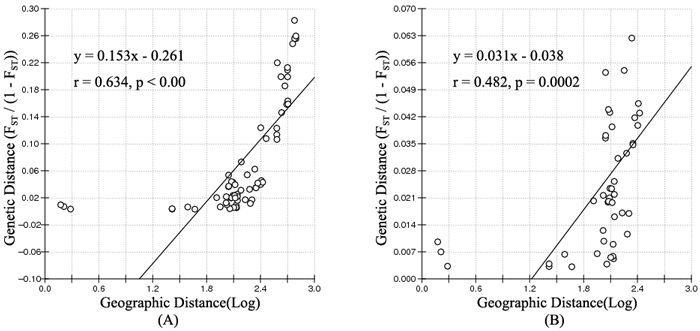
Fig. 4. Isolation By Distance (IBD) analysis between FST/(1–FST) and log (geographic distance) among 12 Salix viminalis populations (A) and among 10 populations in Ergun basin (B).
| Table 3. Analysis of Molecular Variance (AMOVA) of 12 Salix viminalis populations. | |||||
| Source of variation | Degrees of freedom | Sum of squares | Mean Squares | Estimated variance | Explained variance (%) |
| Total populations | |||||
| Between populations | 11 | 382.05 | 34.73 | 0.795 | 6.63 |
| Within populations | 648 | 4506.32 | 13.93 | 6.97 | 93.37 |
| Two clusters (two basins) | |||||
| Between clusters | 1 | 201.40 | 201.40 | 0.93 | 11.49 |
| Between populations within clusters | 10 | 180.65 | 18.07 | 0.19 | 2.38 |
| Within populations | 648 | 4506.33 | 13.93 | 6.97 | 86.13 |
| Two subclusters of Ergun basin | |||||
| Between subclusters | 1 | 59.07 | 59.07 | 0.176 | 2.33 |
| Between populations within subclusters | 8 | 92.88 | 11.61 | 0.066 | 0.88 |
| Within populations | 530 | 3880.71 | 14.67 | 7.34 | 96.80 |
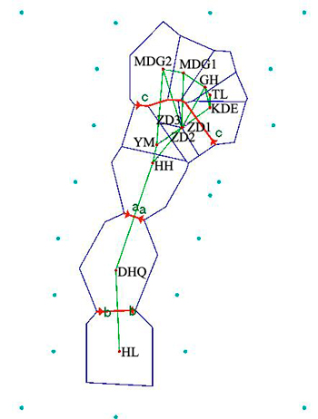
Fig. 5. Genetic barrier of 12 Salix viminalis populations based on Barrier version 2.2. [Note: Abbreviations of populations are explained in Table 1].