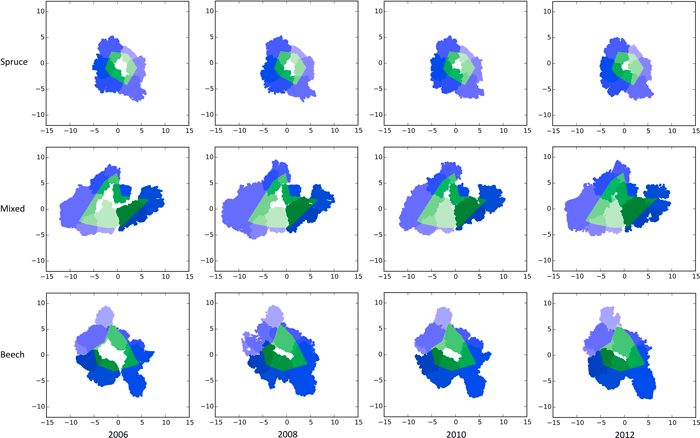
Fig. 1. Bird’s eye view of the TLS scans showing the crown closure from 2006–2012 in pure stands of Norway spruce (top row), a mixed stand of Norway spruce and European beech (middle row) and European beech (bottom row) after generating gaps (white centres) by thinning on the experimental plot FRE 813/1 in 2006. The green areas mark the portion of the crowns lying inside the gap polygon. Blue areas mark the crown regions outside the polygon borders. Different shades of green and blue are given to make the gap’s individual trees visible. View larger in new window/tab.
| Table 1. Individual tree parameters by species from 2006 to 2012. | ||||||||||
| Species | Year | N | DBH [cm] | SE | H [m] | SE | CPAtot [m2] | SE | HCPA [%] | SE |
| Norway spruce | 2006 | 10 | 33.9 | 2.04 | 28.3 | 0.52 | 14.3 | 1.49 | 54.2 | 0.03 |
| 2008 | 10 | 35.0 | 2.03 | 28.6 | 0.50 | 15.1 | 1.24 | 52.1 | 0.02 | |
| 2010 | 10 | 36.1 | 2.06 | 28.8 | 0.48 | 15.9 | 1.05 | 53.4 | 0.03 | |
| 2012 | 10 | 37.1 | 2.04 | 29.0 | 0.46 | 17.8 | 1.12 | 54.0 | 0.03 | |
| European beech | 2006 | 12 | 25.6 | 1.77 | 26.6 | 0.30 | 19.4 | 2.75 | 57.1 | 0.04 |
| 2008 | 12 | 26.1 | 1.80 | 27.0 | 0.30 | 26.3 | 4.12 | 59.0 | 0.05 | |
| 2010 | 12 | 26.4 | 1.82 | 27.3 | 0.31 | 22.0 | 3.22 | 60.1 | 0.04 | |
| 2012 | 12 | 26.7 | 1.83 | 27.6 | 0.31 | 24.4 | 3.62 | 58.3 | 0.04 | |
| N = number of trees, DBH = diameter at breast height, H = height, CPAtot = mean crown projection area derived from two-dimensional α-shapes (α = 0.25 m), HCPA = relative height within crown with maximum projection area, SE = standard error. | ||||||||||
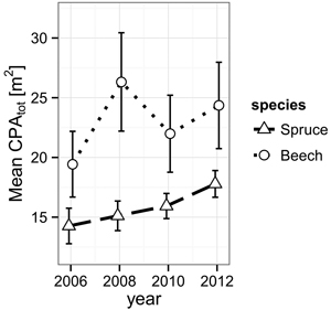
Fig. 2. Development of the mean crown projection area (CPA) derived from α-shapes (α = 0.25 m) of the individual trees’ TLS point clouds for both species from 2006 to 2012. The error bars mark the one-fold standard error.
| Table 2. Allometric parameters. | |||||||
| Species | Year | ADBH | SE | AH | SE | AB | SE |
| Norway spruce | 2008 | 1.39 | 1.01 | 4.40 | 5.52 | 0.67 | 0.51 |
| 2010 | 0.95 | 0.66 | 4.74 | 2.84 | 0.47 | 0.32 | |
| 2012 | 1.56 | 0.44 | 6.97 | 2.64 | 0.77 | 0.22 | |
| European beech | 2008 | 11.02 | 3.75 | 12.60 | 1.95 | 3.74 | 0.99 |
| 2010 | –7.48 | 2.51 | –10.19 | 3.75 | –2.74 | 0.93 | |
| 2012 | 4.18 | 1.10 | 2.14 | 2.96 | –1.54 | 3.06 | |
| ADBH = allocation ratio between crown diameter and DBH, AH = between crown diameter and height, AB = crown diameter and biomass, SE = standard error. | |||||||
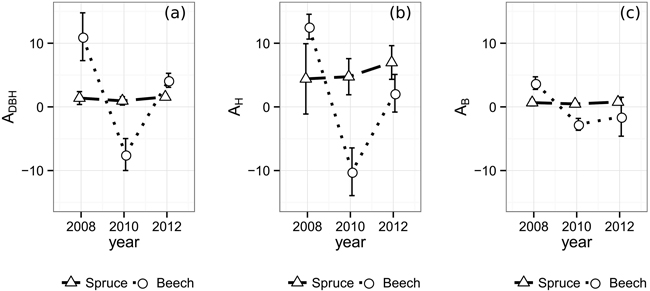
Fig. 3. Allometric relations and one-fold standard error bars over time between (a) crown diameter and DBH, (b) crown diameter and tree height (c) and crown diameter and biomass. In order to take different crown shapes into account, the crown diameter was substituted by the diameter of a hypothetical circle encompassing the same area as its respective tree’s two-dimensional α-shape (α = 0.25 m).
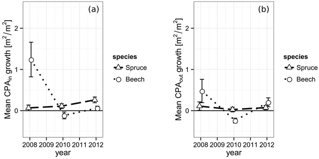
Fig. 4. (a) Increase of the crown projection area by species within the gap polygon, i.e. towards the gap center and (b) increase of the crown projection by species area outside of the gap polygon, towards competing neighbors from 2006 to 2012. The vertical bars indicate the one-fold standard error.
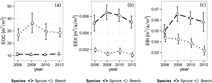
Fig. 5. Development of (a) efficiency of space occupation (EOC), (b) efficiency of space exploitation (EEX) and (c) efficiency of biomass investment (EBI) for each species from 2006 until 2012. Vertical bars indicate the one-fold standard error.
| Table 3. Space utilization parameters by species from 2006 to 2012. View in new window/tab. |
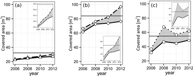
Fig. 6. Layering development of the analyzed (a) spruce, (b) mixed and (c) beech gaps from 2006 until 2012. The solid lines indicate the area of the leaf-cover as a whole. The dashed lines show the sum of all individual tree CPAs forming the respective gap. The difference (gray area) indicates crown overlap, i.e. multi-layering. The black horizontal lines mark the area of the gap polygon, i.e. the highest possible area of the single-layered cover. View larger in new window/tab.
| Table 4. Descriptive data of the gap-level development from 2006–2012. | |||||||
| Gap | Year | Apoly [m2] | GPA [m2] | Rel. closed | ∑CPAin [m2] | ML [m2] | RML |
| Norway spruce | 2006 | 32.2 | 22.6 | 0.70 | 23.15 | 0.55 | 0.02 |
| 2008 | 32.2 | 24.3 | 0.76 | 25.68 | 1.36 | 0.06 | |
| 2010 | 32.2 | 26.1 | 0.81 | 27.27 | 1.15 | 0.04 | |
| 2012 | 32.2 | 27.0 | 0.84 | 30.35 | 3.33 | 0.12 | |
| European beech | 2006 | 54.8 | 32.0 | 0.59 | 36.97 | 4.93 | 0.15 |
| 2008 | 54.8 | 47.0 | 0.86 | 68.02 | 21.00 | 0.44 | |
| 2010 | 54.8 | 44.9 | 0.82 | 56.00 | 12.10 | 0.27 | |
| 2012 | 54.8 | 49.1 | 0.90 | 62.16 | 13.06 | 0.27 | |
| Mixed | 2006 | 84.0 | 61.6 | 0.73 | 66.31 | 4.75 | 0.08 |
| 2008 | 84.0 | 72.5 | 0.86 | 76.19 | 3.68 | 0.05 | |
| 2010 | 84.0 | 73.8 | 0.88 | 82.24 | 8.46 | 0.11 | |
| 2012 | 84.0 | 76.4 | 0.91 | 96.91 | 20.54 | 0.27 | |
| Apoly = area of gap polygon, GPA = gap projection area, ∑CPAin = sum of all crown sections reaching into the gap polygon, ML = multi-layered area, RML = ML in relation to GPA. | |||||||