| Table 1. Samples of broadleaved species. Time series measurements are in bold. Time series measurements were used only when analyzing the seasonal variations in the spectra. | ||||||||
| Species | Location | Date(s) | N trees | Tree height, m | Canopy positions* | N samples per each canopy position in a tree | Leaf sides** | N measured spectra |
| Acer platanoides | Otaniemi | 8.7.2016 | 2 | 6.2, 13.2 | E/S | 3 | A/B | 24 |
| Alnus glutinosa | Otaniemi | 8.7.2016 | 2 | 13.6, 22.1 | E/S | 3 | A/B | 24 |
| Alnus incana | Otaniemi | 6.7.2016 | 2 | 6.2, 18.0 | E/S | 3 | A/B | 24 |
| Betula papyrifera | Kumpula | 12.7.2016 | 2 | 13.7, 17.1 | E/S | 3 | A/B | 24 |
| Betula pendula | Otaniemi | 16.–17.5.2016 | 3 | 5.6, 6.1, 7.2 | E/S | 3 | A/B | 36 |
| 20.5.2016 | 1 | 7.2 | E/S | 3 | A/B | 12 | ||
| 2.-3.6.2016 | 3 | 5.6, 6.1, 7.2 | E/S | 3 | A/B | 36 | ||
| 29.6.2016 | 3 | 5.6, 6.1, 7.2 | E/S | 3 | A/B | 36 | ||
| 28.7.2016 | 3 | 5.6, 6.1, 7.2 | E/S | 3 | A/B | 36 | ||
| 25.8.2016 | 3 | 5.6, 6.1, 7.2 | E/S | 3 | A/B | 36 | ||
| 7.10.2016 | 3 | 5.6, 6.1, 7.2 | E/S | 3 | A/B | 36 | ||
| Populus balsamifera | Kumpula | 12.7.2016 | 1 | 4.8 | E | 12 | A/B | 24 |
| Populus tremula | Otaniemi | 17.5.2016 | 3 | 8.2, 8.9, 10.3 | E/S | 3 | A/B | 36 |
| 20.5.2016 | 1 | 8.2 | E/S | 3 | A/B | 12 | ||
| 2.-3.6.2016 | 3 | 8.2, 8.9, 10.3 | E/S | 3 | A/B | 36 | ||
| 29.–30.6.2016 | 3 | 8.2, 8.9, 10.3 | E/S | 3 | A/B | 36 | ||
| 28.–29.7.2016 | 3 | 8.2, 8.9, 10.3 | E/S | 3 | A/B | 36 | ||
| 25.8.2016 | 3 | 8.2, 8.9, 10.3 | E/S | 3 | A/B | 36 | ||
| 10.7.2016 | 3 | 8.2, 8.9, 10.3 | E/S | 3 | A/B | 36 | ||
| Populus tremuloides | Ruotsinkylä | 21.7.2016 | 1 | 17.8 | E/S | 6 | A/B | 24 |
| Prunus padus | Otaniemi | 8.7.2016 | 2 | 8.5, 9.1 | E/S | 3 | A/B | 24 |
| Quercus robur | Otaniemi | 6.7.2016 | 2 | 3.1, 21.6 | E/S | 3 | A/B | 24 |
| Salix caprea | Otaniemi | 4.7.2016 | 2 | 11.9, 16.7 | E/S | 3 | A/B | 24 |
| Sorbus aucuparia | Otaniemi | 6.7.2016 | 2 | 11.5, 13.0 | E/S | 3 | A/B | 24 |
| Tilia cordata | Viikki | 24.8.2016 | 2 | 5.8, 16.7 | E/S | 3 | A/B | 24 |
| * E = Sun-exposed, S = shaded ** A = adaxial, B = abaxial | ||||||||
| Table 2. Samples of coniferous species. Time series measurements are in bold. These were only used when analyzing the seasonal variations in the spectra. | |||||||||
| Species | Location | Date(s) | N trees | Tree height, m | Canopy positions* | Age cohorts** | N samples per each canopy position and age cohort in a tree | Needle sides*** | N measured spectra |
| Abies balsamea | Viikki | 20.7., 17.8.2016 | 2 | 11.1¸12.7 | E/S | c0/c1 | 3 | A/B | 48 |
| Abies sibirica | Viikki | 23.8.2016 | 1 | 23.7 | E/S | c0/c1 | 3 | A/B | 24 |
| Larix gmelinii | Viikki | 4.8.2016 | 1 | 14.1 | E/S | c0 | 6 | A/B | 24 |
| Larix laricina | Viikki | 22.8.2016 | 1 | 16.7 | E/S | c0 | 6 | A/B | 24 |
| Larix sibirica | Viikki | 3.8.2016 | 1 | 26.7 | S | c0 | 12 | A/B | 24 |
| Picea abies | Otaniemi | 14.–23.6.2016 | 2 | 16.4, 22.6 | E/S | c0/c1 | 3 | - | 24 |
| 26.7.–1.8.2016 | 2 | 16.4, 22.6 | E/S | c0/c1 | 3 | - | 24 | ||
| 12.–13.9.2016 | 2 | 16.4, 22.6 | E/S | c0/c1 | 3 | - | 24 | ||
| Picea glauca | Viikki | 30.8.2016 | 2 | 11.4, 14.9 | E/S | c0/c1 | 3 | - | 24 |
| Picea mariana | Viikki | 18.–19.8.2016 | 2 | 8.4, 9.0 | E/S | c0/c1 | 3 | - | 24 |
| Pinus banksiana | Viikki | 19.8., 24.8.2016 | 1 | 13.7 | E/S | c0/c1 | 6 | A/B | 48 |
| Pinus contorta | Viikki | 18.7., 17.8.2016 | 2 | 17.1, 19.7 | E/S | c0/c1 | 3 | A/B | 48 |
| Pinus sylvestris | Otaniemi | 17.–22.6.2016 | 2 | 13.3, 14.2 | E/S | c0/c1 | 3 | A/B | 48 |
| 22.–25.7.2016 | 2 | 13.3, 14.2 | E/S | c0/c1 | 3 | A/B | 48 | ||
| 12.–14.9.2016 | 2 | 13.3, 14.2 | E/S | c0/c1 | 3 | A/B | 48 | ||
| Pseudotsuga menziesii | Viikki | 11.7., 16.8.2016 | 2 | 20.7, 26.2 | E/S | c0/c1 | 3 | A/B | 48 |
| * E = Sun-exposed, S = shaded ** c0 = current year needles, c1 = previous year needles *** A = adaxial, B = abaxial | |||||||||
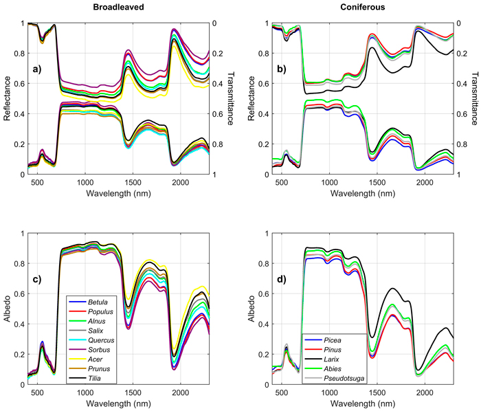
Fig. 1. Mean reflectance, transmittance, and albedo spectra by genus in broadleaved (a,c) and coniferous (b,d) trees. View larger in new window/tab.
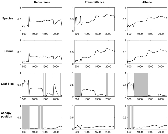
Fig. 2. Coefficients of determination (R2) when variability of reflectance, transmittance, and albedo spectra of broadleaved tree leaves were explained by species, genus, leaf side (adaxial/abaxial), and canopy position (sun-exposed/shaded) in one-way ANOVA. Statistically non-significant regions (p > 0.05) are highlighted in gray. The x-axis denotes wavelength (nm) and y-axis coefficient of determination (0–1).
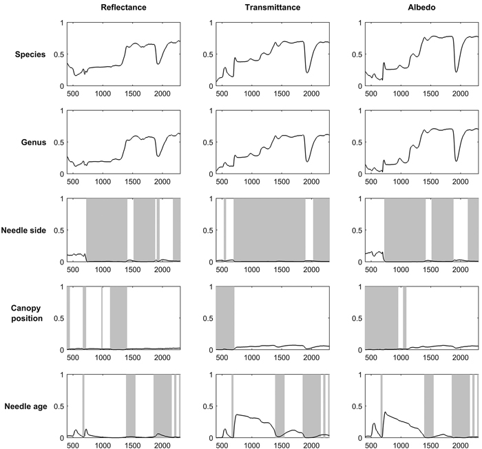
Fig. 3. Coefficients of determination (R2) when variability in reflectance, transmittance, and albedo spectra of coniferous needles were explained by species, genus, needle side (adaxial/abaxial), and canopy position (sun-exposed/shaded) in one-way ANOVA. Statistically non-significant regions (p > 0.05) are highlighted in gray. The x-axis denotes wavelength (nm) and y-axis coefficient of determination (0–1).
| Table 3. Coefficients of determination (R2) when variability of red edge inflection point (REIP) were explained by species, genus, leaf or needle side (adaxial/abaxial), canopy position (sun-exposed/shaded), and needle age in one-way ANOVA. Corresponding p-value is given in brackets. | |||
| REIP (reflectance) | REIP (transmittance) | REIP (albedo) | |
| Broadleaved | |||
| Species | 0.12 (0.00) | 0.24 (0.00) | 0.23 (0.00) |
| Genus | 0.07 (0.00) | 0.12 (0.00) | 0.09 (0.00) |
| Leaf side | 0.45 (0.00) | 0.03 (0.00) | 0.16 (0.00) |
| Canopy position | 0.02 (0.03) | 0.07 (0.00) | 0.07 (0.00) |
| Coniferous | |||
| Species | 0.45 (0.00) | 0.67 (0.00) | 0.61 (0.00) |
| Genus | 0.29 (0.00) | 0.46 (0.00) | 0.41 (0.00) |
| Leaf side | 0.14 (0.00) | 0.00 (0.70) | 0.02 (0.01) |
| Canopy position | 0.00 (0.84) | 0.00 (0.38) | 0.00 (0.39) |
| Needle age | 0.07 (0.00) | 0.11 (0.00) | 0.09 (0.00) |
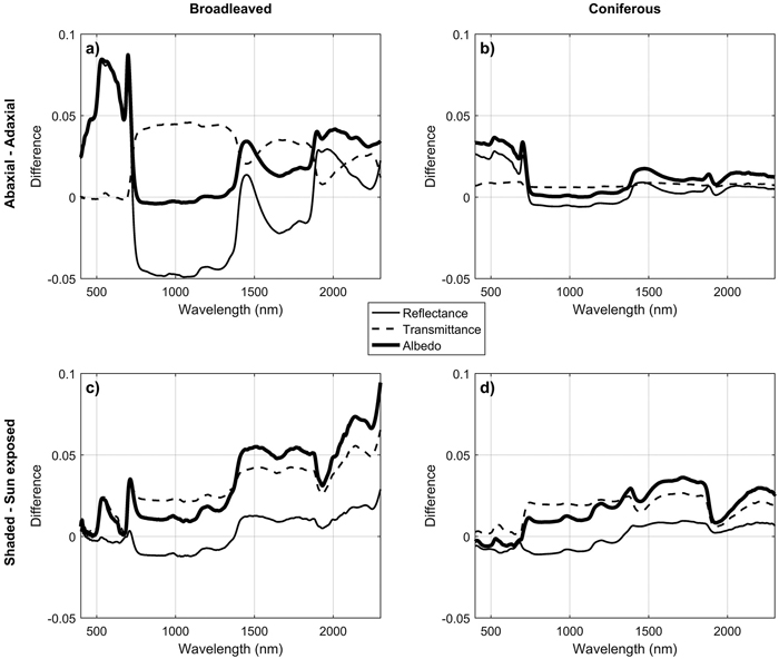
Fig. 4. Mean spectral differences between abaxial vs. adaxial sides of leaves and needles (a,b) and between shaded vs. sun-exposed canopy positions (c,d).
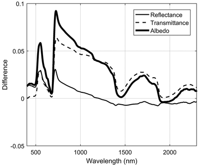
Fig. 5. Spectral differences between two age cohorts of coniferous needles (new i.e. current year – previous year).
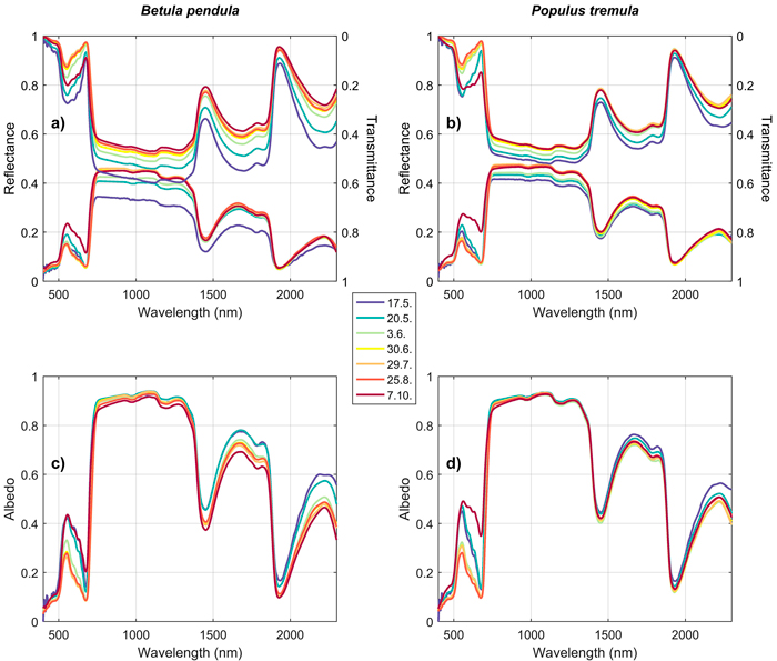
Fig. 6. Seasonal trends in silver birch (Betula pendula) (a,c) and European aspen (Populus tremula) (b,d) reflectance, transmittance, and albedo spectra. The color denotes time of measurement (last day if the measurements were obtained within two days). View larger in new window/tab.
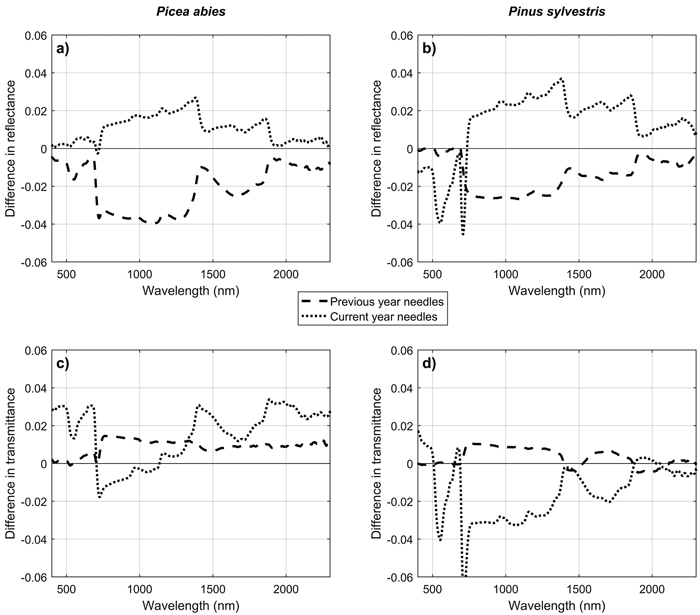
Fig. 7. Differences in mean reflectance (a,b) and transmittance (c,d) of Scots pine (Pinus sylvestris) and Norway spruce (Picea abies) needles between June and September. Difference was calculated as (mean in September – mean in June), separately for current year and previous year needles.