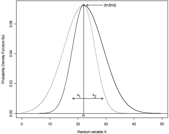
Fig. 1. A sample graph of the double normal distribution with m = 22, s1 = 4 and s2 = 7. Notation: m – the mean of the compound distributions that becomes an overall distribution mode, s1 – the standard deviation of the first compound distribution, which makes a left half of the overall distribution, s2 – the standard deviation of the second compound distribution, which makes a right half of the overall distribution; solid lines show the resulting double normal distribution.
| Table 1. Summary statistics of the 20 sample plots used in the study. |
| | Area | Age | N | QMD | MD | HL | BA | SI |
| [ha] | [years] | [trees] | [cm] | [cm] | [m] | [m2 ha–1] | [m] |
| Minimum | 0.049 | 26 | 258 | 6.2 | 5.9 | 7.70 | 22.40 | 16.90 |
| Maximum | 0.810 | 123 | 500 | 28.7 | 28.3 | 23.20 | 31.20 | 27.20 |
| Average | 0.297 | 58 | 378 | 15.5 | 15.0 | 14.34 | 27.18 | 22.03 |
| Std dev. | 0.235 | 25 | 67 | 6.0 | 5.9 | 3.70 | 2.55 | 3.53 |
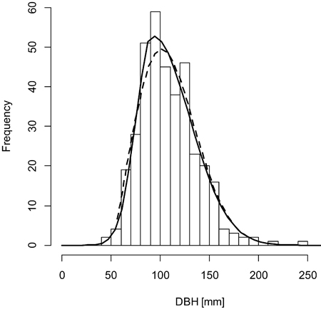
Fig. 2. A sample graph of the double normal distribution (solid line) outperforming the Weibull distribution (dashed line) for the plot BT119 (histogram).
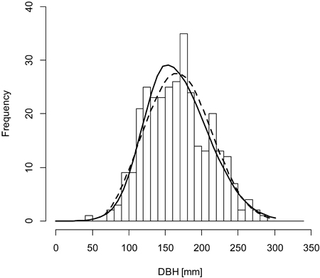
Fig. 3. A sample graph of the Weibull distribution (dashed line) outperforming the double normal distribution (solid line) for the plot BT130 (histogram).
| Table 2. Detailed values of the Dn statistics for various distributions and methods of fitting. MLE denotes the maximum likelihood method, MOM3 – method of moments based on first three moments of the sample, MOM2 – method of moments based on first two moments of the sample and the distribution mode estimated using the approximate formula: mode = mean – 4.8 · (mean – median), MOM2W – method of moments based on first two moments of the sample. Lower value of the Dn statistics denote better fit. The best fit is marked with bold numbers. |
| | | Double normal | Weibull |
| Plot | MLE | MOM3 a) | MOM2 a) | MLE | MOM2W |
| BT112 | 0.0356 | 0.0327 | 0.0327 | 0.0324 | 0.0317 |
| BT113 | 0.0347 | 0.0285 | 0.0285 | 0.0294 | 0.0282 |
| BT114 | 0.0452 | 0.0542 | 0.0542 | 0.0568 | 0.0613 |
| BT115 | 0.0391 | 0.0490 | 0.0490 | 0.0373 | 0.0412 |
| BT116 | 0.0385 | 0.0413 | 0.0413 | 0.0422 | 0.0428 |
| BT117 | 0.0344 | 0.0355 | 0.0355 | 0.0380 | 0.0378 |
| BT118 | 0.0453 | 0.0294 | 0.0294 | 0.0255 | 0.0249 |
| BT119 | 0.0244 | 0.0399 | 0.0399 | 0.0384 | 0.0343 |
| BT120 | 0.0572 | 0.0396 | 0.0396 | 0.0345 | 0.0321 |
| BT121 | 0.0277 | 0.0441 | 0.0441 | 0.0379 | 0.0375 |
| BT122 | 0.0317 | 0.0355 | 0.0355 | 0.0310 | 0.0310 |
| BT123 | 0.0315 | 0.0310 | 0.0310 | 0.0212 | 0.0211 |
| BT124 | 0.0253 | 0.0197 | 0.0197 | 0.0275 | 0.0271 |
| BT125 | 0.0221 | 0.0261 | 0.0261 | 0.0474 | 0.0406 |
| BT126 | 0.0394 | 0.0476 | 0.0476 | 0.0552 | 0.0462 |
| BT127 | 0.0322 | 0.0283 | 0.0283 | 0.0264 | 0.0302 |
| BT128 | 0.0340 | 0.0323 | 0.0323 | 0.0289 | 0.0298 |
| BT129 | 0.0391 | 0.0349 | 0.0349 | 0.0397 | 0.0386 |
| BT130 | 0.0361 | 0.0354 | 0.0354 | 0.0273 | 0.0277 |
| BT131 | 0.0499 | 0.0390 | 0.0390 | 0.0315 | 0.0270 |
| Avg. | 0.0362 | 0.0362 | 0.0362 | 0.0354 | 0.0346 |
| Table 3. Detailed values of the Dn statistics and number of cases when the hypothesis about matching the empirical and theoretical distributions was rejected for various distributions and methods of fitting for 100 samples of 50 trees. For explanations of the abbreviations see Table 2. MLE(S) – the maximum likelihood method with simulated annealing optimization algorithm. The best fit without MLE(S) method is marked with bold numbers, and with the MLE(S) – with underlined numbers. |
| Plot | Double normal | Weibull |
| MLE | 0.05 | MLE(S) | 0.05 | MOM3 | 0.05 | MOM2 | 0.05 | MLE | 0.05 | MOM2W | 0.05 |
| BT112 | 0.0973 | 7 | 0.0753 | 0 | 0.0811 | 0 | 0.0890 | 0 | 0.0674 | 0 | 0.0660 | 0 |
| BT113 | 0.0967 | 8 | 0.0715 | 0 | 0.0698 | 0 | 0.0756 | 0 | 0.0670 | 0 | 0.0652 | 0 |
| BT114 | 0.1054 | 7 | 0.0845 | 4 | 0.1533 | 0 | 0.0859 | 0 | 0.0855 | 1 | 0.0894 | 0 |
| BT115 | 0.0906 | 2 | 0.0798 | 2 | 0.0985 | 0 | 0.0793 | 0 | 0.0802 | 0 | 0.0771 | 0 |
| BT116 | 0.1329 | 12 | 0.0752 | 0 | 0.0733 | 0 | 0.0789 | 0 | 0.0670 | 0 | 0.0729 | 0 |
| BT117 | 0.1352 | 14 | 0.0773 | 0 | 0.0867 | 0 | 0.0847 | 0 | 0.0757 | 0 | 0.0752 | 0 |
| BT118 | 0.1168 | 9 | 0.0773 | 1 | 0.0691 | 0 | 0.0741 | 0 | 0.0697 | 0 | 0.0711 | 0 |
| BT119 | 0.1078 | 6 | 0.0776 | 0 | 0.1251 | 0 | 0.0910 | 0 | 0.0789 | 0 | 0.0781 | 0 |
| BT120 | 0.1563 | 18 | 0.0799 | 0 | 0.0877 | 0 | 0.0900 | 0 | 0.0758 | 0 | 0.0794 | 0 |
| BT121 | 0.1193 | 12 | 0.0720 | 0 | 0.0753 | 0 | 0.0791 | 0 | 0.0687 | 1 | 0.0706 | 0 |
| BT122 | 0.1738 | 20 | 0.0735 | 0 | 0.0785 | 0 | 0.0776 | 0 | 0.0660 | 0 | 0.0690 | 0 |
| BT123 | 0.1794 | 22 | 0.0726 | 0 | 0.0890 | 0 | 0.0753 | 0 | 0.0627 | 0 | 0.0608 | 0 |
| BT124 | 0.1350 | 15 | 0.0718 | 1 | 0.0978 | 0 | 0.0693 | 0 | 0.0703 | 2 | 0.0683 | 0 |
| BT125 | 0.0756 | 2 | 0.0857 | 1 | 0.0743 | 0 | 0.0726 | 0 | 0.0768 | 1 | 0.0747 | 0 |
| BT126 | 0.0825 | 1 | 0.0750 | 1 | 0.0896 | 0 | 0.0819 | 0 | 0.0889 | 2 | 0.0914 | 0 |
| BT127 | 0.0838 | 2 | 0.0709 | 0 | 0.0783 | 0 | 0.0829 | 0 | 0.0723 | 0 | 0.0700 | 0 |
| BT128 | 0.1013 | 5 | 0.0740 | 0 | 0.0778 | 0 | 0.0830 | 0 | 0.0684 | 0 | 0.0748 | 0 |
| BT129 | 0.0971 | 5 | 0.0735 | 0 | 0.0855 | 0 | 0.0886 | 0 | 0.0769 | 1 | 0.0683 | 0 |
| BT130 | 0.0946 | 5 | 0.0767 | 0 | 0.0697 | 0 | 0.0774 | 0 | 0.0716 | 0 | 0.0743 | 0 |
| BT131 | 0.1133 | 8 | 0.0780 | 0 | 0.0912 | 0 | 0.0829 | 0 | 0.0727 | 0 | 0.0769 | 0 |
| Avg. | 0.1147 | | 0.0761 | | 0.0876 | | 0.0809 | | 0.0731 | | 0.0737 | |
| Table 4. Detailed values of the Dn statistics and number of cases when the hypothesis about matching the empirical and theoretical distributions was rejected for various distributions and methods of fitting for 100 samples of 10 trees. For explanations of the abbreviations see Table 2. The best fit is marked with bold numbers. |
| Plot | Double normal | Weibull |
| MLE | 0.05 | MLE(S) | 0.05 | MOM3 | 0.05 | MOM2 | 0.05 | MLE | 0.05 | MOM2W | 0.05 |
| BT112 | 0.3519 | 45 | 0.1857 | 6 | 0.1678 | 1 | 0.1755 | 1 | 0.1472 | 0 | 0.1391 | 0 |
| BT113 | 0.3210 | 37 | 0.2050 | 12 | 0.1555 | 2 | 0.1562 | 1 | 0.1387 | 0 | 0.1379 | 1 |
| BT114 | 0.4111 | 53 | 0.2461 | 15 | 0.2076 | 4 | 0.1735 | 0 | 0.1577 | 0 | 0.1590 | 1 |
| BT115 | 0.3605 | 39 | 0.1953 | 4 | 0.1823 | 2 | 0.1675 | 0 | 0.1482 | 0 | 0.1529 | 0 |
| BT116 | 0.3478 | 40 | 0.1891 | 3 | 0.1745 | 2 | 0.1698 | 1 | 0.1394 | 0 | 0.1408 | 0 |
| BT117 | 0.3947 | 50 | 0.2154 | 9 | 0.1894 | 4 | 0.1786 | 3 | 0.1528 | 2 | 0.1466 | 0 |
| BT118 | 0.3348 | 38 | 0.1868 | 3 | 0.1530 | 2 | 0.1556 | 1 | 0.1478 | 0 | 0.1407 | 2 |
| BT119 | 0.3604 | 44 | 0.2275 | 7 | 0.1867 | 3 | 0.1722 | 3 | 0.1536 | 0 | 0.1499 | 1 |
| BT120 | 0.4047 | 50 | 0.2154 | 7 | 0.1698 | 3 | 0.1708 | 2 | 0.1510 | 1 | 0.1466 | 0 |
| BT121 | 0.3522 | 42 | 0.2059 | 3 | 0.1690 | 1 | 0.1724 | 1 | 0.1290 | 0 | 0.1358 | 0 |
| BT122 | 0.4264 | 56 | 0.1979 | 9 | 0.1782 | 2 | 0.1688 | 0 | 0.1473 | 0 | 0.1362 | 1 |
| BT123 | 0.3514 | 39 | 0.2031 | 9 | 0.1742 | 1 | 0.1567 | 1 | 0.1419 | 0 | 0.1382 | 1 |
| BT124 | 0.3946 | 50 | 0.1671 | 2 | 0.1657 | 1 | 0.1576 | 0 | 0.1325 | 0 | 0.1350 | 0 |
| BT125 | 0.3530 | 40 | 0.1739 | 4 | 0.1642 | 2 | 0.1677 | 2 | 0.1611 | 0 | 0.1485 | 1 |
| BT126 | 0.3227 | 36 | 0.1791 | 3 | 0.1806 | 3 | 0.1619 | 0 | 0.1636 | 0 | 0.1536 | 0 |
| BT127 | 0.3840 | 49 | 0.1700 | 0 | 0.1451 | 0 | 0.1478 | 0 | 0.1565 | 0 | 0.1488 | 0 |
| BT128 | 0.3413 | 38 | 0.1839 | 1 | 0.1616 | 5 | 0.1607 | 3 | 0.1626 | 1 | 0.1402 | 0 |
| BT129 | 0.3259 | 35 | 0.1923 | 6 | 0.1644 | 2 | 0.1725 | 1 | 0.1648 | 0 | 0.1388 | 0 |
| BT130 | 0.3322 | 38 | 0.1894 | 7 | 0.1716 | 2 | 0.1812 | 1 | 0.1668 | 1 | 0.1447 | 2 |
| BT131 | 0.3324 | 36 | 0.1849 | 4 | 0.1669 | 1 | 0.1636 | 1 | 0.1586 | 2 | 0.1524 | 2 |
| Avg. | 0.3602 | | 0.1958 | | 0.1714 | | 0.1665 | | 0.1511 | | 0.1443 | |