| Table 1. The main characteristics of the study stands. | ||||||
| Study site | Study trail | Number of sample plots | Volume of trees, Vplot m3/ha | Stem density n/ha | Dry mass of logging residues kg/ha | Site type a) |
| 1 | 1 | 4 | 104 | 1865 | 17200 | Vatkg |
| 1 | 2 | 4 | 64 | 1350 | 9100 | Vatkg |
| 1 | 3 | 4 | 79 | 1688 | 9100 | Vatkg |
| 1 | 4 | 4 | 76 | 1103 | 9500 | Vatkg |
| 2 | 1 | 3 | 160 | 1193 | 21700 | Ptkg |
| 2 | 2 | 4 | 130 | 1302 | 17300 | Ptkg |
| 2 | 3 | 4 | 129 | 1760 | 15500 | Ptkg |
| 2 | 4 | 4 | 112 | 1307 | 13500 | Ptkg |
| 2 | 5 | 4 | 115 | 960 | 13700 | Ptkg |
| 2 | 6 | 4 | 122 | 1060 | 11400 | Ptkg |
| 3 | 1 | 4 | 184 | 1497 | 31000 | Ptkg |
| 3 | 2 | 4 | 126 | 1142 | 20600 | Ptkg |
| 3 | 3 | 4 | 170 | 1360 | 28600 | Ptkg |
| 3 | 4 | 4 | 139 | 1228 | 22100 | Ptkg |
| a) Site type classification according to Laine and Vasander (2005). | ||||||
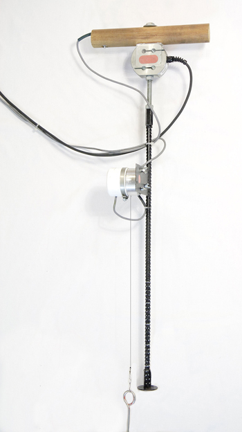
Fig. 1. Manually operated plate loading device.
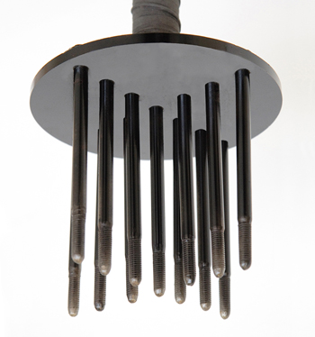
Fig. 2. Spiked shear vane for measuring the shear modulus of the root layer of peatland.
| Table 2. Technical data for the machines used in the study. | ||||
| Equipment | John Deere 1270D harvester | John Deere 1110D forwarder | ProSilva 15-4ST forwarder | |
| Front axle | Number of wheels | 4 | 4 | - |
| Tyres | 710/40-22.5 | 710/45-26.5 | - | |
| Tracks | Clark Terra TL-85 | Clark Terra TL85 | excavator type | |
| Track width, mm | 730 | 780 | 810 | |
| Length of track soil contact on hard ground, mm | 2200 | |||
| Net mass with tracks or chains, kg | 10160 | 12280 | 9140 | |
| NGP, kPa | 50 | 52 | 25 | |
| Rear axle | Number of wheels | 2 | 4 | |
| Tyres | 650/60-26.5 | 710/45-26.5 | ||
| Tracks | Terra-X TXL150 | excavator type | ||
| Track width, mm | (wheel chains) | 887 | 810 | |
| Length of track soil contact on hard ground, mm | 2700 | |||
| Net mass with tracks or chains, kg | 7240 | 9940 | 10120 | |
| Mass of load, kg | - | 8500 | 8000 | |
| NGP, kPa (unloaded/loaded) | 74 | 32/59 | 23/41 | |
| Table 3. Means of the main factors of the peat land in the study trails. Gpoint = Shear modulus of measurement point, Epoint = Modulus of elasticity of measurement point, CPRpoint = Cone penetration resistance of measurement point, VWCpoint = Volumetric water content of measurement point, GWT = Ground water table level, Peat depth = Depth of peat layer and Shrubsplot = Coverage of mire dwarf shrubs within the plot. | ||||||||
| Study site | Study trail | Gpoint | Epoint | CPRpoint | VWCpoint | GWT | Peat depth | Shrubsplot |
| Mean (std.dev.) KPa | Mean (std. dev.) KPa | Mean (std. dev.) KPa | Mean (std. dev.) % | Mean cm | Mean cm | Mean % | ||
| 1 | 1 | 43.1 | 91.3 | 271 | 55.4 | 41 | 290 | 26.3 |
| 2 | 39.5 | 111 | 249 | 57.0 | - | 269 | 15.0 | |
| 3 | 44.2 | 232 | 60.3 | - | 284 | 38.6 | ||
| 4 | 40.2 | 89.1 | 237 | 49.1 | 40.3 | |||
| All | 41.8 (15.8) | 96.8 (33.4) | 247 (89.1) | 55.5 (11.5) | 40.6 | 286 | 29.4 | |
| 2 | 1 | 45.6 | 95.0 | 392 | 45.1 | 65.7 | 138 | 33.3 |
| 2 | 35.4 | 62.7 | 159 | 37.0 | 60.8 | 155 | 20.0 | |
| 3 | 31.8 | 69.6 | 219 | 44.4 | 59.0 | 166 | 18.3 | |
| 4 | 47.5 | 93.2 | 257 | 33.9 | 57.8 | 198 | 13.8 | |
| 5 | 47.5 | 93.2 | 265 | 43.1 | 59.5 | 171 | 16.3 | |
| 6 | - | - | 253 | 47.4 | 62.0 | 164 | 22.5 | |
| All | 37.0 (18.1 | 76.5 (35.4) | 251 (110) | 41.7 (16.2) | 60.3 | 167 | 20.2 | |
| 3 | 1 | 37.1 | 75.0 | 343 | 37.3 | - | 190 | 22.5 |
| 2 | 30.9 | 41.4 | 252 | 37.6 | - | 206 | 8.75 | |
| 3 | 48.3 | 75.9 | 317 | 43.1 | - | 188 | 10.0 | |
| 4 | 36.4 | 93.9 | 289 | 40.4 | - | 178 | 12.5 | |
| All | 38.2 (16.4) | 71.6 (37.1) | 300 (138) | 39.6 (9.26) | 68.4 | 190 | 13.4 | |
| All | 38.9 (16.9) | 81.4 (36.8) | 265 (116) | 45.1 (14.7) | 58.0 | 208 | 20.9 | |
| Table 4. Means of rut depths by study trails. RutHarvplot = Mean of rut depths caused by harvester within the sample plot and RutForwplot = Mean of rut depths after one harvester pass, one forwarder pass unloaded and one forwarder pass loaded within the sample plot. For study site 1, study plots with (Brash mat = 1) and without brash mat (Brash mat = 0) are given separately. | |||||
| Study site | Study trail | Brash mat | Forwarder type | RutHarvplot cm | RutForwplot cm |
| 1 | 1 | 1 | Tracked forwarder | 10.4 | 12.1 |
| 0 | Tracked forwarder | 18.6 | 22.9 | ||
| 2 | 1 | 11.1 | - | ||
| 0 | 18.5 | - | |||
| 3 | 1 | 13.8 | - | ||
| 0 | 29.4 | - | |||
| 4 | 1 | Tracked forwarder | 9.6 | 15.8 | |
| 0 | Tracked forwarder | 19.1 | 26.9 | ||
| 2 | 1 | 1 | Tracked forwarder | 7.0 | 9.0 |
| 2 | 1 | Wheeled forwarder | 11.7 | 17.7 | |
| 3 | 0 | Wheeled forwarder | 23.7 | 32.3 | |
| 4 | 0 | Tracked forwarder | 24.1 | 24.4 | |
| 5 | 1 | Wheeled forwarder | 8.2 | 17.8 | |
| 6 | 1 | 7.5 | |||
| 3 | 1 | 1 | 8.7 | - | |
| 2 | 0 | 13.8 | - | ||
| 3 | 0 | Tracked forwarder | 13.6 | 17.7 | |
| 4 | 1 | Tracked forwarder | 13.5 | 16.0 | |
| Mean | 12.5 | 17.7 | |||
| Table 5. Correlation coefficients between rut depth, mechanical properties of peat soil and factors affecting the mechanical properties. P-values and number of observations are given in the rows below the coefficient. Values printed in bold indicate significant correlation. Vplot = Volume of trees within the plot, Peat depth = Depth of peat layer, Shrubsplot = Coverage of mire dwarf shrubs within the plot, VWCplot = Mean of volumetric water content within the plot, CPRplot = Mean of cone penetration resistance within the plot, Eplot = Mean of modulus of elasticity within the plot, Gplot = Mean of shear modulus within the plot, RutHarvplot = Mean of rut depths caused by harvester within the sample plot with brash mat (Brash mat = 1) and without brash mat (Brash mat = 0). | |||||||||
| Vplot (m3/ha) | Peat depth (cm) | Shrubsplot (%) | VWCplot (%) | CPRplot (KPa) | Eplot (KPa) | Gplot (KPa) | RutHarvplot Brash mat = 0 (m) | RutHarvplot Brash mat = 1 (m) | |
| Vplot (m3/ha) | 1 | –0.571 0.000 55 | –0.205 0.133 55 | –0.476 0.000 55 | 0.281 0.038 55 | –0.357 0.010 | –0.065 0.650 51 | –0.451 0.018 27 | –0.171 0.395 28 |
| Peat depth (cm) | 1 | 0.297 0,028 55 | 0.555 0.000 55 | –0.083 0.548 55 | 0.364 0.009 51 | 0.157 0.270 51 | 0.407 0.035 27 | –0.008 0.968 28 | |
| Shrubsplot (%) | 1 | 0.411 0.002 55 | –0.021 0.878 55 | 0.264 0.061 51 | 0.194 0.174 51 | 0.060 0.764 27 | –0.037 0.855 28 | ||
| VWCplot (%) | 1 | –0.120 0.382 55 | 0.563 0.000 51 | 0.382 0.006 51 | 0.329 0.093 27 | –0.125 0.533 28 | |||
| CPRplot (kPa) | 1 | 0.233 0.100 55 | 0.203 0.153 55 | –0.465 0.014 27 | –0.134 0.506 28 | ||||
| Eplot (kPa) | 1 | 0.507 0.000 51 | –0.046 0.819 27 | –0.065 0.764 28 | |||||
| Gplot (kPa) | 1 | –0.282 0.155 27 | –0.456 0.025 28 | ||||||
| RutHarvplot Brash mat = 0 (m) | 1 | 0 | |||||||
| RutHarvplot Brash mat = 1 (m) | 1 | ||||||||
| Table 6. Mixed-linear models predicting rut depths after one harvester pass (RutHarvijkl). N = 255. Gpoint = Shear modulus of measurement point, Vplot = Volume of trees within the plot, VWCpoint = Volumetric water content of measurement point, Brash mat is a binary variable that takes the value 1 in the case study plot has brash mat and 0 in the case study plot has no brash mat, “ * ” is the symbol of multiplication, var(ujkl) = variance of the plot, var(vkl) = variance of trail, var(yl) = variance of site, var(eijkl) = residual variance and AIC = Akaike’s Information Criterion. | ||||||
| Model | 1 | 2 | 3 | |||
| Parameter | Estimate (SE) | Sig. | Estimate (SE) | Sig. | Estimate (SE) | Sig. |
| Fixed | ||||||
| Intercept | 32.7 (12.4) | .013 | 39.6 (13.3) | .001 | –224 (107) | .038 |
| lnGpoint | –1.59 | .210 | 70.9 (29.7) | .018 | ||
| lnVplot | –4.68 (2.57) | .078 | –4.93 (2.52) | .060 | 25.9 (15.6) | .098 |
| lnVWCpoint | 31.4 (14.8) | .035 | ||||
| lnVplot * lnGpoint | –8.48 (4.22) | .046 | ||||
| lnGpoint * lnVWCpoint | –8.63 (4.15) | .039 | ||||
| [Brash mat = 0] | 9.09 (1.63) | .000 | 8.87 (1.61) | .000 | 9.04 (1.61) | .000 |
| [Brash mat = 1] | 0 | 0 | 0 | |||
| Random | ||||||
| var(ujkl) | 11.7 (4.52) | .010 | 11.2 (4.43) | .005 | 10.9 (4.31) | .012 |
| var(vkl) | 7.24 (4.90) | .140 | 7.00 (4.66) | 7.06 (4.76) | .138 | |
| var(yl) | .000 | .000 | .000 | |||
| var(eijkl) | 38.6 (3.82) | .000 | 38.6 (3.83) | .000 | 37.6 (3.73) | .000 |
| AIC | 1728.2 | 1728.6 | 1728.3 | |||
| Table 7. Mixed-linear models predicting rut depths after one harvester pass and two forwarder passes (RutForvijkl). N = 165. Gpoint = Shear modulus of measurement point, Vplot = Volume of trees within the plot, VWCpoint = Volumetric water content of measurement point, Brash mat is a binary variable that takes the value 1 in the case study plot has brash mat and 0 in the case study plot has no brash mat, Forwarder type is a binary variable that takes the value “Wheeled forwarder” in the case of the John Deere and “Tracked forwarder” in the case of the Prosilva, “ * ” is the symbol of multiplication, var(ujkl) = variance of the plot, var(vkl) = variance of trail, var(yl) = variance of site, var(eijkl) = residual variance and AIC = Akaike’s Information Criterion. | ||||||
| Model | 1 | 2 | 3 | |||
| Parameter | Estimate (SE) | Sig. | Estimate (SE) | Sig. | Estimate (SE) | Sig. |
| Fixed | ||||||
| Intercept | 52.9 (17.6) | .006 | 69.9 (20.0) | .001 | 70.2 (17.6) | .000 |
| lnGpoint | –4.51 (1.63) | .006 | ||||
| lnVplot | –8.23 (3.65) | .032 | –8.88 (3.62) | .020 | –8.40 (3.40) | .020 |
| lnVWCpoint | –3.67 (2.33) | .088 | ||||
| [Brash mat = 0] * [Forwarder type = “Wheeled forwarder”] | 19.3 (3.77) | .000 | 19.3 (3.72) | .000 | 18.0 (3.73) | .000 |
| [Brash mat = 0] * [Forwarder type = ”Tracked Forwarder”] | 8.54 (2.41) | .001 | 8.36 (2.37) | .001 | 8.12 (2.25) | .001 |
| [Brash mat = 1] * [Forwarder type = ”Wheeled forwarder”] | 4.45 (2.67) | .106 | 4.05 (2.65) | .137 | 4.41 (2.49) | .087 |
| [Brash mat = 1] * [Forwarder type = ”Tracked Forwarder”] | 0 | 0 | 0 | |||
| Random | ||||||
| var(ujkl) | 23.6 (8.72) | .006 | 22.7 (8.50) | .008 | 19.3 (7.70) | .012 |
| var(vkl) | .000 | .000 | .000 | |||
| var(yl) | .000 | .000 | .000 | |||
| var(eijkl) | 46.3 (5.70) | .007 | 45.9 (5.67) | .000 | 45.5 (6.16) | .000 |
| AIC | 1128.4 | 1022.1 | 1018.2 | |||