| Table 1. Three thinning treatments tested at each site, 1) heavy thinning, 2) ordinary thinning and 3) light thinning. Means for tree height (H), stem number (N), basal area (BA) and tree diameter (Dg, tree of mean basal area) refer to the situation prior to thinning. | |||||||||||||
| Site 1 – Järpås | |||||||||||||
| Year | Stand age (yrs) | Heavy thinning | Ordinary thinning | Light thinning | |||||||||
| H (m) | N (stems ha–1) | BA (m2 ha–1) | Dg (cm) | H (m) | N (stems ha–1) | BA (m2 ha–1) | Dg (cm) | H (m) | N (stems ha–1) | BA (m2 ha–1) | Dg (cm) | ||
| 2002 | 9 | 8.9 | 2433 | 12.2 | 8.0 | 9.0 | 2429 | 12.5 | 8.1 | 8.7 | 2407 | 12.2 | 8.0 |
| 2007 | 14 | 15.2 | 726 | 10.5 | 13.6 | 14.9 | 1154 | 14.3 | 12.6 | 14.7 | 1566 | 17.1 | 11.8 |
| 2012 | 19 | 18.7 | 711 | 15.3 | 16.6 | 18.4 | 804 | 15.8 | 15.8 | 17.8 | 990 | 16.7 | 14.7 |
| Site 2 – Bökö | |||||||||||||
| 2003 | 10 | 2053 | 2103 | 2138 | |||||||||
| 2008 | 15 | 13.5 | 804 | 9.9 | 12.5 | 12.8 | 1260 | 12.2 | 11.1 | 12.7 | 1577 | 14.5 | 10.8 |
| 2010 | 17 | 14.7 | 804 | 11.7 | 13.6 | 13.9 | 1260 | 14.0 | 11.9 | 14.4 | 1106 | 14.0 | 12.7 |
| 2014 | 21 | 16.6 | 804 | 15.9 | 15.7 | 16.7 | 809 | 15.1 | 15.4 | 16.4 | 1106 | 18.9 | 14.7 |
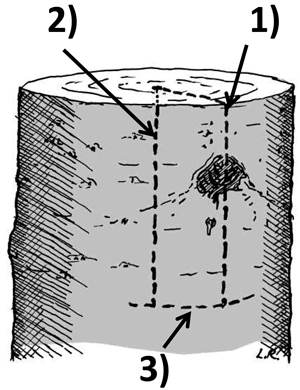
Fig. 1. Illustration of how the knot samples were produced. A vertical cut with a chain saw was directed through the centre of the knot towards the pith (1). A second vertical cut directed towards the pith was made a few cm from the first (2). A third cut released the sample, shaped like a slice of cake. Picture taken from Rytter and Jansson (2009).
| Table 2. Description of traits. Illustrations are presented in Fig. 2. | ||
| Trait | Unit | Description |
| CardP | N, E, S, W | Cardinal point of the twig. Every twig was designated to one of the four points. |
| KnAng | Degrees (90°) | Knot angle from a horizontal line (Fig. 2, no 2) |
| Radius | mm | Horizontal distance from pith to trunk surface, excluding the protuberance, (Fig. 2, no 5 in the lower illustration) |
| Dia | mm | Tree diameter at 13 dm above ground in autumn 2012 (age 19) at site 1 and 2014 (age 21) at site 2 |
| TwHght | cm | Height from ground to the twig |
| KnDia | mm | Diameter of the knot at the outer end or trunk edge (Fig. 2, no 1) |
| Dist1 | mm | Length of new wood with wood defects (Fig. 2, no 3) |
| Dist2 | mm | Length of defect-free new wood (Fig. 2, no 4) |
| Dist3 | mm | Total length of new wood (Dist1 + Dist2) |
| BrkUp | mm | Length of ingrown bark above the knot (cf. BrkLow) |
| BrkLow | mm | Length of ingrown bark below the knot (Fig. 2, no 6) |
| ColIn | % | Proportion of wood discolouration within the knot (Fig. 2, no A) |
| ColOut | % | Proportion of wood discolouration outside the knot (Fig. 2, no B) |
| RotIn | % | Proportion of wood rot within the knot (Fig. 2, no A) |
| RotOut | % | Proportion of wood rot outside the knot (Fig. 2, no B) |
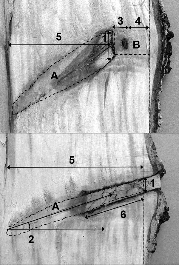
Fig. 2. Example of measurements of traits in pruned (top picture) and unpruned (bottom picture) trees: 1 = vertical knot thickness; 2 = knot angle; 3 = discoloured wood and wood with rot in the horizontal direction; 4 = defect-free wood outside the knot; 5 = distance from pith to knot end; 6 = length of ingrown bark; A = area within the knot from which areas affected by discolouration and rot were estimated as a percentage; B = area between knot end and vertical trunk edge (excluding the protuberance commonly found outside a twig) from which areas affected by discolouration and rot were estimated as a percentage.
| Table 3. Number of observations (N), arithmetic means (Mean), standard deviations (Std), minimum (Min) and maximum (Max) values for different traits at each site, based on individual knot/twig data. Description of traits are given in Table 2. | |||||||||||
| Trait | Unit | Site = 1 (Järpås) | Site = 2 (Bökö) | ||||||||
| N | Mean | Std | Min | Max | N | Mean | Std | Min | Max | ||
| Dia | mm | 335 | 141 | 20.0 | 102 | 179 | 348 | 138 | 18.7 | 91 | 273 |
| Radius | mm | 335 | 59 | 8.8 | 38 | 84 | 348 | 54 | 7.9 | 33 | 73 |
| TwHght | cm | 335 | 238 | 37.0 | 150 | 300 | 348 | 240 | 37.8 | 140 | 300 |
| KnDia | mm | 335 | 12.1 | 5.8 | 2 | 40 | 348 | 10.8 | 6.7 | 2 | 55 |
| KnAng | ° | 335 | 42 | 9.1 | 7 | 64 | 348 | 41 | 10.2 | 11 | 65 |
| Dist1 | mm | 335 | 0.9 | 1.9 | 0 | 12 | 348 | 0.7 | 1.7 | 0 | 10 |
| Dist2 | mm | 335 | 9.1 | 8.1 | 0 | 32 | 348 | 6.0 | 6.8 | 0 | 30 |
| Dist3 | mm | 335 | 10.1 | 8.1 | 0 | 32 | 348 | 6.6 | 7.2 | 0 | 30 |
| BrkUp | mm | 335 | 11.1 | 11.4 | 0 | 66 | 348 | 18.9 | 23.6 | 0 | 105 |
| BrkLow | mm | 335 | 5.3 | 5.7 | 0 | 32 | 348 | 6.1 | 6.9 | 0 | 35 |
| ColIn | % | 335 | 30 | 14.7 | 0 | 90 | 348 | 29 | 18.2 | 0 | 100 |
| ColOut | % | 335 | 4.9 | 12.0 | 0 | 90 | 348 | 4.0 | 13.0 | 0 | 100 |
| RotIn | % | 335 | 7.9 | 9.5 | 0 | 40 | 348 | 11.5 | 11.9 | 0 | 100 |
| RotOut | % | 335 | 0.0 | 0.0 | 0 | 0 | 348 | 0.7 | 6.4 | 0 | 100 |
| Table 4. Statistical results for difference in pruning treatments and least-square means of pruned and unpruned trees for different traits for each site (Eq. 1) and for both sites (Site 1 + 2, Eq. 2). A “x” in the column “Covar” indicates the result when the covariate KnDia was included in Eq. 1 and 2. Bold figures are significant at the 5%-level. Description of traits are given in Table 2. View in new window/tab. |
| Table 5. Correlations between different traits at site 1. Bold figures are significant at the 5% level. Description of traits are given in Table 2. | |||||||||
| Trait | KnAng | Dist1 | Dist2 | Dist3 | BrkUp | BrkLow | ColIn | ColOut | RotIn |
| KnDia | 0.52 | 0.15 | –0.22 | –0.18 | 0.14 | 0.01 | 0.24 | 0.14 | 0.07 |
| KnAng | 0.06 | –0.04 | –0.03 | 0.34 | –0.11 | 0.06 | 0.05 | –0.01 | |
| Dist1 | –0.11 | 0.13 | 0.07 | 0.06 | 0.13 | 0.75 | 0.06 | ||
| Dist2 | 0.97 | 0.03 | –0.07 | 0.22 | –0.18 | –0.13 | |||
| Dist3 | 0.05 | –0.05 | 0.25 | 0.00 | –0.11 | ||||
| BrkUp | 0.27 | 0.11 | 0.05 | 0.33 | |||||
| BrkLow | 0.04 | 0.09 | 0.48 | ||||||
| ColIn | 0.15 | –0.23 | |||||||
| ColOut | 0.09 | ||||||||
| Table 6. Correlations between different traits at site 2. Bold figures are significant at the 5% level. Description of traits are given in Table 2. | |||||||||
| Trait | KnAng | Dist1 | Dist2 | Dist3 | BrkUp | BrkLow | ColIn | ColOut | RotIn |
| KnDia | 0.40 | 0.07 | –0.09 | –0.07 | 0.13 | –0.25 | 0.05 | –0.02 | 0.09 |
| KnAng | –0.02 | –0.13 | –0.13 | 0.41 | –0.20 | –0.12 | –0.02 | –0.15 | |
| Dist1 | 0.12 | 0.36 | –0.10 | 0.04 | 0.08 | 0.69 | 0.11 | ||
| Dist2 | 0.97 | –0.16 | –0.09 | 0.18 | 0.00 | 0.02 | |||
| Dist3 | –0.17 | –0.07 | 0.19 | 0.17 | 0.04 | ||||
| BrkUp | 0.20 | 0.22 | –0.10 | 0.11 | |||||
| BrkLow | 0.42 | 0.10 | 0.53 | ||||||
| ColIn | 0.07 | 0.64 | |||||||
| ColOut | 0.09 | ||||||||