Nils Fahlvik  ,
Björn Elfving,
Peder Wikström
,
Björn Elfving,
Peder Wikström
Evaluation of growth functions used in the Swedish Forest Planning System Heureka
Fahlvik N., Elfving B., Wikström P. (2014). Evaluation of growth functions used in the Swedish Forest Planning System Heureka. Silva Fennica vol. 48 no. 2 article id 1013. https://doi.org/10.14214/sf.1013
Highlights
- Growth models based on historical growth data gave reliable growth predictions up to the century shift
- Detailed single tree growth models had lower precision for estimation of total growth than one single stand-based model
- The prediction error was in average about 15% and did not increase with extended prediction period.
Abstract
The performance of growth models implemented in the Swedish Forest Planning System Heureka was evaluated. Four basal area growth models were evaluated by comparing their predictions to data from five-year growth records for 1711 permanent sample plots of the National Forest Inventory (NFI-data). Also, two alternative implementations of Heureka, including a combined stand- and tree-level basal area growth model and a single tree-level model, respectively, were evaluated using data from 57 blocks in a thinning experiment (GG-data) involving Scots pine (Pinus sylvestris L.) and Norway spruce (Picea abies (L.) Karst) in which the trees were monitored for 30 years after the first thinning. The predicted volume growth was also compared to observed values. Growth models based on data from 1970’s and 1980’s overestimated growth in the NFI test plots from the early 2000’s by about 3%. Stand-level models had larger precision than tree-level models. Basal area growth was underestimated in dense NFI-plots and overestimated in non-thinned GG-plots, illustrating an un-solved modelling problem. Basal area growth was overestimated by 2–5% also in the GG-plots over the whole observation period. Volume growth was however accurately predicted for pine and underestimated by 2% for spruce. The relative prediction error did not increase with increasing length of prediction period. Thinning response models calibrated with GG-data worked well in the total application and produced growth levels for different thinning alternatives in line with observations.
Keywords
basal area;
simulation;
validation;
volume;
empirical
-
Fahlvik,
Department of Southern Swedish Forest Research Centre, Swedish University of Agricultural Sciences, P.O. Box 49, SE-230 53 Alnarp, Sweden
E-mail
nils.fahlvik@slu.se
- Elfving, Department of Forest Ecology and Management, Swedish University of Agricultural Sciences, SE-901 83 Umeå, Sweden E-mail bjorn.elfving@slu.se
- Wikström, Peder Wikström Skogsanalys AB, c/o Peder Wikström, Huldrans väg 1, SE-907 52 Umeå, Sweden E-mail peder.wikstrom@slu.se
Received 3 October 2013 Accepted 11 March 2014 Published 7 May 2014
Views 166044
Available at https://doi.org/10.14214/sf.1013 | Download PDF

1 Introduction
Forest growth simulators are important tools in practical forestry and forest research, with applications ranging from forest planning to evaluating silvicultural measures and assessing changes in growth conditions. While simulators and models were initially used to study even-aged monocultures under traditional management, there is an increasing demand for growth simulators that can handle more diverse forest structures and treatments (Teuffel et al. 2006). Due to the increasing number of growth simulators and the wider range of situations in which they can be applied, there is a need for reliable documentation of the different simulators’ performance under various conditions and for documentation that will enable users to apply them correctly and with confidence (e.g. Vanclay and Skovsgaard 1997; Pretzsch et al. 2002).
The development of the Hugin forest planning system and its successor Heureka prompted the construction of various empirical growth models that have found widespread use in modern Swedish forestry (Hägglund 1981; Elfving 2010a; Wikström et al. 2011). These models describe two key stages in stand growth: the stand establishment period and the development of the established stand. The transition between the two stages typically occurs at an average stand height of 7–8 m. The stand-level growth models of Ekö (1985) and Elfving (2010a) and the tree-level growth models of Söderberg (1986) and Elfving (2010a) were developed for predicting attributes of established forests across Sweden and can be applied to forests containing any of the major tree species found within the country. All of these models for established forests were developed using data from the National Forest Inventory (NFI).
The key advantage of tree-level models relative to their stand-level counterparts is that they can be used to estimate both the yield distribution of a stand as a function of species and tree size as well as the stand’s total yield (which is obtained by aggregating the estimates for individual trees). However, stand-level models are considered to predict stand attributes more reliably (Mäkinen et al. 2008; Yue et al. 2008). Various authors have therefore proposed that by using the two model types in tandem, it might be possible to develop a system that combines the high resolution of tree-level models with the simplicity and robustness of stand-level models (Qin and Cao 2006; Yue et al. 2008). The Heureka system was designed with this concept, using tree-level growth models to model yield distributions and one single stand-level model for calibrating overall stand growth.
Heureka was developed for use in long-term forest planning (Wikström et al. 2011). It was designed for planning both on the regional-, ownership- and stand-level and involves tools to handle economic values, silvicultural treatments and harvesting, timber production, forest fuels, biodiversity and carbon sequestration. It is distributed as a free-ware tool and has won a wide-spread use. Most of the larger forest owners in Sweden use it.
A common problem encountered in the long-term forecasting of growth and yield is the decreasing accuracy of the estimates with increasing prognosis length (Holm 1981; Kangas 1997). This is partly because forecasts are made recursively, with the independent variables typically being updated every fifth year. As a result, the magnitude of the errors in the estimated independent variables increases in each successive forecast period (Kangas 1997).
The annual growth in Swedish forests has increased from about 80 million m3 around 1970 to about 115 million m3 around 2005. The increased growth is probably mainly an effect of changed silviculture but also increased nitrogen deposition and concentration of greenhouse gases in the air are assumed to have increased growth (Elfving and Tegnhammar 1996). An important question is then if growth models based on historic growth can give reliable predictions of future growth.
The aim of the study reported herein was to assess the reliability of growth predictions generated by Heureka through comparison to observed growth in established stands. The specific hypotheses tested were:
- Growth models based on historic data will underestimate future growth
- Single-tree growth models give more accurate predictions than stand-level models
- The precision of the growth predictions decrease with increased projection period
Heureka’s growth simulator includes a large set of sub-models for predicting site and stand data (e.g. site index, tree age), growth and mortality. This evaluation focused on the sub-models used for estimating growth, including tree- and stand-level basal area growth, tree-level height growth, and volume growth based on estimated tree diameter and height data. Basal area growth models are the central components of the Heureka system. Consequently, the first stage of our analysis involved comparing predictions using those basal area growth models to recent data from permanent NFI plots. The performance of selected alternative growth models developed for use in Sweden was also tested. The NFI-data were used to compare the performance of the growth models over a wide range of site and stand types. In the second stage, estimates of basal area and volume growth generated by long-term Heureka simulations were compared to observations from a nation-wide thinning experiment. The purpose of the second stage was to study the influence of recursive forecast periods on accuracy and the ability to predict growth responses to a wide range of thinning treatments. Long-term growth simulations were performed with both the default configuration of Heureka (which uses a linked set of tree- and stand-level basal area growth models) and an alternative configuration that uses tree-level models exclusively. It must be stressed that available test data sets were not totally independent of calibration data. This will be more detailed in the discussion of the results.
2 Material and methods
2.1 Evaluation of basal area growth models using NFI-data
2.1.1 NFI-data
The NFI-data used for evaluation were obtained by measuring trees growing on permanent plots (Ranneby et al. 1987) established between 1983 and 1987. Around 18 500 such plots were established in total; their locations were chosen so as to provide a representative sample of forests throughout Sweden. The plots are arranged in grids, with those in the south being denser than those in the north. In plots with a radius of 10 m, all trees whose diameter at breast height (DBH; 1.3 m above ground) was greater than 99 mm at the start of the growth period were monitored individually. Smaller trees were measured in different ways on sub-plots of different sizes and thus could not be considered in this work. Our study dealt with non-divided plots on productive forest land with mean stand heights above 8 m. To facilitate analysis, plots in which trees with a DBH > 99 mm had been thinned or had died of natural causes during the observation period were also excluded. In total, 1711 plots that satisfied the criteria outlined above were selected for analysis in this study (Table 1). On average, Scots pine (Pinus sylvestris L.) accounted for 45% of the total basal area considered, Norway spruce (Picea abies (L.) Karst) for 37%, birch (Betula sp.) for 13% and other tree species for 5%. Data from five-year measurement campaigns conducted during 1999–2004, 2000–2005, 2001–2006, and 2002–2007 were used. During each measurement campaign, the trees’ DBH values were determined in mm using a calliper. The species and status (alive, dead, removed or missing) of each tree examined was also recorded.
| Table 1. Site and initial stand characteristics of the 1711 selected National Forest Inventory permanent plots. | ||||||
| Site index a) (m) | Stand age b) (years) | Diameter at breast height b) (cm) | Mean height b) (m) | Basal area (m2 ha–1) | No. of stems ha–1 | |
| Average | 21.7 | 79 | 20.6 | 15.5 | 21.2 | 2526 |
| Min | 8.0 | 17 | 5.7 | 8.0 | 0.5 | 32 |
| 5%-percentile | 13.0 | 25 | 10.6 | 8.5 | 8.1 | 318 |
| 95%-percentile | 32.0 | 155 | 33.5 | 24.0 | 38.3 | 7669 |
| Max | 38.0 | 255 | 59.7 | 35.0 | 61.7 | 28482 |
| Stdv | 5.7 | 42 | 7.3 | 4.9 | 9.3 | 2841 |
| a) Site index (H100) calculated based on site factors for Scots pine and Norway spruce, respectively (Hägglund and Lundmark 1977) b) Basal area weighted mean (ƩX×d2 / Ʃd2) | ||||||
Observations on the permanent NFI-plots were nominally conducted over five growing seasons. However, since the first and second measurements were typically performed at different time points during the growing season, the observed DBH growth was corrected for deviation from the nominal observation period. The correction was carried out by estimating the fraction of DBH growth achieved at a specific time during the growing season, assuming a sigmoidal growth pattern (cf. Valinger 1992; Söderberg et al. 1993).
2.1.2 Models for estimating basal area growth
The evaluation focused on two stand-level models developed by Ekö (1985) (OLD_S) and Elfving (2010a) (NEW_S) and two tree-level models developed by Söderberg (1986) (OLD_T) and Elfving (2010a) (NEW_T).
The OLD_S and OLD_T growth models were developed using data acquired between 1973 and 1977 from temporary plots measured by the NFI (Svensson 1980). Growth rates were determined by measuring the last five year rings in increment cores from representative sample trees. Stand data five years before the measurements were reconstructed from increment cores of standing trees and from estimated properties of dead and removed trees based on stump analysis. OLD_S includes models that estimate growth ha–1 values for a range of species including Scots pine, Norway spruce, birch, European beech (Fagus sylvatica (L.)), oak (Quercus sp.), and other broad-leaved trees, with separate models for different parts of the country and different site index classes. OLD_T incorporates separate models for different regions and for different age groups of the above-mentioned tree species.
The NEW_S and NEW_T growth models were based on data from the first observation period on the permanent plots established by the NFI in 1983–1987 (Ranneby et al. 1987). Growth was registered in terms of the difference between calliper measurements performed at five year intervals. NEW_S uses one single model to estimate the total growth ha–1 for all tree species. NEW_T incorporates separate models for Scots pine, Norway spruce, birch, European aspen (Populus tremula (L.)), European beech, oak, and other noble and trivial broad-leaved species. The group “noble” include ash (Fraxinus excelsior (L.)), maple (Acer platanoides (L.)), lime (Tilia cordata (Mill.)) and elm (Ulmus glabra (Huds.)). The group “trivial” include alder (Alnus sp.), rowan (Sorbus acuparia (L.)) and willows (Salix sp).
All of the tested models are empirical and generate five-year growth estimates based on independent input variables describing the site (e.g. latitude, altitude, site index) and the stand (e.g. stand age, density and time since thinning). The models used in OLD_T and NEW_T rely on input variables that describe the properties of individual trees (e.g. species and diameter), and their competitive status as expressed by their position in the diameter distribution. These models also include expressions for the overall density of the studied plot. The largest differences between OLD_T and NEW_T are the totally different error structures for the dependent variable (ring width measurements on increment cores, difference in callipered diameter at start and end of the growth period), the large difference in precision of age determination (age at breast height of single trees according to ring counting on increment cores, total stand age estimated in the field) and the representation of competitive status for single trees (relative tree diameter, basal area of larger trees). Another large difference between the OLD_S / OLD_T models and the NEW_S / NEW_T models is the number of estimated parameters. The former models were split on age- and site-classes and contain each between 400–600 estimated parameters while the latter models use continuous variables to express influence by age and site conditions. The NEW_S model only contains 19 estimated parameters.
The evaluated growth models require input data on stand age or the ages of individual trees. These data were obtained using age-models for individual trees developed by Elfving (2003) on the basis of NFI-data. The site index was defined as expected top height of the stand at a total age of 100 years (H100), and site index values for Norway spruce and Scots pine were estimated for each plot according to the properties of each site (Hägglund and Lundmark 1977).
2.2 Long-term test of Heureka
2.2.1 Data from long-term thinning experiments (GG-data)
Data from a nationwide thinning experiment that focused on monocultures of Scots pine and Norway spruce (Nilsson et al. 2010, Table 2) were used to evaluate the accuracy of long-term simulations using Heureka. The so called GG-experiment was established between 1966 and 1983 to study the effects of thinning (Gallring) and fertilization (Gödsling) treatments on growth and yield. The thinning treatments examined included different thinning grades, thinning forms and timings of first thinning. In total, single blocks with 6–12 treatments were established on 48 sites with Scots pine and 23 with Norway spruce. The Scots pine sites were distributed widely across the country whereas the Norway spruce sites were concentrated in Central and Southern Sweden.
| Table 2. Initial site and stand characteristics of the 57 blocks from the thinning experiment used for evaluating long-term Heureka simulations. | |||||||
| Latitude | Site index a) | Basal area (m2 ha–1) | No. of stems ha–1 | Top height (m) | Stand age (years) | ||
| Scots pine | Average | 21.3 | 24.1 | 2151 | 13.4 | 41.0 | |
| Min | 56°23´N | 14.8 | 14.6 | 1295 | 11.8 | 32.0 | |
| 40 blocks | Max | 67°29´N | 26.9 | 36.3 | 3585 | 15.4 | 58.0 |
| Stdv | 3.4 | 4.65 | 542 | 1.07 | 6.47 | ||
| Norway spruce | Average | 29.6 | 32.8 | 3136 | 13.8 | 29.8 | |
| Min | 56°06´N | 22.0 | 23.7 | 1346 | 12.6 | 23.0 | |
| 17 blocks | Max | 63°14´N | 32.3 | 39.0 | 4931 | 16.2 | 37.0 |
| Stdv | 2.6 | 4.90 | 1009 | 1.01 | 3.86 | ||
| a) Site index (H100) according to site factors (Hägglund and Lundmark 1977) | |||||||
Data from six treatments applied to the Scots pine and Norway spruce plots were used in this study. Four of these treatments involved thinning from below with different thinning grades and intensities (treatments A, B, C and D), one involved thinning from above (F), and the last was an non-thinned control (I) (definitions and nomenclature according to Nilsson et al. 2010) (Table 3). Treatment C involved only one heavy thinning. In treatments A, B, D and F, the basal area after thinning was maintained at approximately the same level after all thinnings, increasing slightly over time. The treatments based on thinning from below focused on removing trees with smaller dimensions. Conversely, during thinning from above, the dominant tree classes were removed preferentially. However, at least some trees from all diameter classes were removed under both thinning regimes in order to promote the optimal development of those trees remaining in the stand. For treatments A, B, and D, the thinning quotient (i.e. the ratio of the mean DBH value for the removed trees to that for the retained trees) increased slowly over successive thinnings, whereas the opposite was true for treatment F. No fertilizer was applied in any of the treatments considered. Only the 40 Scots pine and 17 Norway spruce sites that had undergone at least three rounds of thinning were considered (Table 3). The time between the first and the last measurements for Scots pine plots varied from 19 to 41 years, with an average of 30 years. For Norway spruce plots, the average time between the first and the last measurement was 28 years, with a range of 18 to 35 years. The only treatments for which the data set contained a complete set of plots were A, C, F and I for Scots pine, and A, C and I for Norway spruce.
| Table 3. Description of the thinning treatments used in the experiments that provided the data against which the Heureka simulations were evaluated. | |||||||
| Species | Treatment | Number of plots | No. of thinnings | First thinning | |||
| Thinning grade a) (%) | Thinning quotient b) | Basal area after thinning (m2 ha–1) | No. of stems ha–1 after thinning | ||||
| Scots pine | A | 40 | 3–4 | 25.5 | 0.73 | 17.9 | 1265 |
| B | 16 | 2–3 | 43.1 | 0.73 | 13.0 | 869 | |
| C | 40 | 1 | 59.4 | 0.73 | 9.6 | 563 | |
| D | 16 | 3–4 | 50.6 | 0.72 | 11.7 | 760 | |
| F | 40 | 3–4 | 24.3 | 1.16 | 18.1 | 1743 | |
| I | 40 | 0 | |||||
| Norway spruce | A | 17 | 3–6 | 22.3 | 0.71 | 25.2 | 1992 |
| B | 15 | 2–3 | 40.3 | 0.72 | 19.7 | 1408 | |
| C | 17 | 1 | 64.8 | 0.72 | 11.1 | 684 | |
| D | 9 | 4–6 | 43.9 | 0.71 | 19.4 | 1405 | |
| F | 10 | 3–5 | 20.8 | 1.18 | 25.8 | 2580 | |
| I | 17 | 0 | |||||
| a) Percentage of basal area removed b) Ratio of the diameters of removed and retained trees | |||||||
The plots covered an area of 0.1 ha on average and were surrounded by buffer zones. Measurements were conducted at the start of the experiment, during every thinning and also periodically between thinnings. All DBH values were cross-callipered at a permanently marked position on the stem. The species, status (retained, removed, missing, wind-felled) and properties (damage, vitality) of each studied tree were also recorded on each measurement occasion, along with the heights of selected sample trees. The site index (H100) for each experimental site was estimated based on site factors as described by Hägglund and Lundmark (1977).
2.2.2 Growth simulation in Heureka
The Heureka system has been described in general terms by Wikström et al. (2011), and Elfving (2010a) has described the procedures used for growth modelling in more detail. The system requires input data comprising information on one or more sample plots and all of the relevant factors affecting them. Specifically, for each plot there should be a list of all trees with DBH values of 4 cm or more, including the species and measured diameter of every such tree. Other required input data include the mean age of the trees within the plot, the latitude and altitude of the site on which the plot is located, the nature of the field vegetation present, soil moisture, site index and details concerning the thinning regime applied. Breast height ages for individual trees are estimated using models developed by Elfving (2003) and the time to reach breast height is estimated using a model that assimilates data from a table compiling NFI field measurements that have been recorded since 1983. Stands to be modelled must also be classified as being either even- or uneven-aged; even-aged stands are defined as stands in which > 80% of the stand volume comes from trees whose ages are within the same 20-year range. Stand development is predicted over a series of five-year stages. Heureka allows the user to choose which models are used in growth simulations. By default, basal area growth is estimated at both the tree-level, using models for single trees (NEW_T), and for the whole stand using a stand-level model (NEW_S). In the combined model (HEU_NEW), the latter model is used to calibrate the growth level while the individual-tree models are used to model how this overall growth is distributed between the various trees present. In this work, we tested both the default configuration and an optional configuration (HEU_OLD) that uses only tree-level models for prediction of basal area growth (OLD_T). Height growth is predicted using top-height development models (Elfving 2010a). The height H2 at age A2 is estimated as a function of the initial height H1 and age A1 (cf. Elfving and Kiviste 1997). Height growth predicted with this model is adjusted according to the competitive situation for each tree as expressed by the basal area of larger trees. By default, stem volumes are estimated using models developed by Brandel (1990). Thinning responses are predicted using special models based on GG-data (Elfving 2010a).
Measurements acquired when the experiment was established were used as the starting point for the simulation; these measurements provided data on all living trees present within the studied plots before the application of any thinning regime. Throughout the simulation period, the list of trees used in the simulation remained identical to those observed in the field. Trees that were removed during thinning or found to have died between measurement periods in the experiment were removed from the simulation at the corresponding point in its timeline.
The initial heights for all trees were used as input data in the Heureka simulations and were estimated using height curves. For each plot, sample trees were used to parameterize the model for the diameter-height relationship (the height curve) proposed by Näslund (1936) for Scots pine and Pettersson (1955) for Norway spruce. The heights for all other trees were then estimated from their DBH values using the appropriate height curve.
Stem volumes for individual trees were estimated using models developed by Brandel (1990). In the experiments, the stem volumes of the sample trees were estimated and these estimated volumes were used in conjunction with equations describing the relationships between basal area and volume to estimate the volume of every callipered tree in each diameter class. The resulting volumes were summed to yield a total volume according to the method described in detail by Nilsson et al. (2010). In Heureka, the individual stem volumes estimated on basis of predicted height and diameter for each tree are simply summed to estimate the overall stand volume.
The mean annual observed and estimated basal area increment (iG) for each plot was calculated for each measurement occasion using the following expression:

where BAt is the basal area for all categories (including retained, removed and dead trees); BAr is the basal area of retained living trees; T is the time since the establishment of the experiment; i is an index running over the re-measurement occasions; n is the number of re-measurements, inclusive of the current measurement occasion. The mean annual increment in the total stem volume (iV) for each plot and measurement occasion was calculated analogous to that shown in Eq. 1.
The growth models and the different configurations of the Heureka system evaluated in this study are summarized in Table 4.
| Table 4. Summary of the evaluated basal area growth models and the alternative implementations of growth models in the Heureka system. | |||
| Name | Basal area growth model | Level | Remarks |
| Growth models | |||
| OLD_S | Ekö (1985) | Stand | Temporary NFI plots 1973–1977 |
| OLD_T | Söderberg (1986) | Tree | Temporary NFI plots 1973–1977 |
| NEW_S | Elfving (2010a) | Stand | Permanent NFI plots est. 1983–1987 |
| NEW_T | Elfving (2010a) | Tree | Permanent NFI plots est. 1983–1987 |
| Configurations of Heureka | |||
| HEU_OLD | Söderberg (1986) | Tree | OLD_T in use |
| HEU_NEW | Elfving (2010a) | Combined tree-stand | NEW_S+NEW_T in use |
2.3 Statistics
The output of the basal area growth models was compared to the data from the NFI plots both in absolute (2) and relative (3) terms according to:
![]()
![]()
where y is the observed value and ŷ is the estimated value.
Principally the variance of residuals is proportional to the predicted growth and a logarithmic transformation will homogenize the variance and give different observations proper weight in statistical analyses. In addition, large measurement errors were associated with growth estimations by repeated callipering on the NFI plots and negative growth was obtained on some plots. A constant was added to the observed and estimated value before logarithmic transformation in order to avoid negative values without truncation of the distribution and to get a homogenous variance, as shown in Fig. 1.
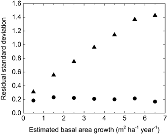
Fig. 1. The standard deviation of residuals by NEW_S for the NFI-data in absolute (res, triangle) and transformed (zres, circle) terms in different classes of estimated growth.
In the GG-data used in these evaluations the measurement errors were negligible and a normal logarithmic transformation could be applied to compare the mean annual increments in basal area and volume in relative terms:
![]()
where y is the observed value and ŷ is the estimated value.
Standard deviations of residuals and relative residuals were used as measures of precision and were estimated as:

where i is an index of plot and n is the total number of plots. The significance of differences between observed and estimated growth were tested in the relative scale, after correction of the differences for logarithmic bias (addition of the value Szres2 / 2). The significance of deviation was tested as t = zresmean / (Szres / √n). The significance of differences in precision was tested as F(1, df 1710) (SSf1 – SSf2) / (SSf2 / df), where SS is sum of squared residuals from compared models f1 and f2.
Residuals of growth were studied to determine how the simulations’ accuracy and precision changed with increasing simulation length. This analysis was performed for treatments A, F and I, since they were considered to be the treatments whose comparison would be most informative. Data from all measurement occasions for each plot within the thinning experiment were used. The maximum length of the observation period varied between the plots. Thus the number of plots used in this study decreased as the number of consecutive simulation periods increased. In order to check trends the residuals were smoothed over the length of observation period with second-degree polynomial using the LOESS procedure of SAS (version 9.3). The effect of error propagation was examined by a study of standard deviation after different length of observation period.
Residuals per plot over the total observation period (observed-estimated growth) were analysed for estimation of accuracy and precision of long-term predictions. The total residual variance was expressed as a function of block (random factor) and treatment (fixed factor) in variance analyses with the MIXED procedure of SAS. The standard deviation of the within-block and between blocks (between stand) variation were calculated from the variance components given by the programme.
3 Results
3.1 Evaluation of basal area growth models using NFI-data
NEW_T underestimated and all other of the studied basal area growth models overestimated the average growth compared to that observed over five years on the NFI plots (Table 5). The greatest deviation in absolute terms was found for OLD_S, with NEW_S and OLD_T giving the least deviation, in absolute terms an overestimation by 3%. The significance of the deviations was evaluated in the relative scale. All deviations but those by OLD_T were significant. There was also a significant variation in deviation (growth level) between measurement periods, Fig. 2.
| Table 5. Basal area growth (iG, m2 ha–1) over a five year period based on observations of permanent National Forest Inventory plots and estimates generated using various basal area growth models. Residuals were calculated in absolute and relative terms. Significant deviation from 0 for relative residuals was marked with (*) (p < 0.001). | ||||||||
| Variable | 5 years basal area growth (m2 ha–1) | Residuals a) (m2 ha–1) | Relative residuals b) | |||||
| Mean | Std.dev. | Mean | Std.dev. | r2 | Mean | Std.dev. | r2 | |
| Observed | 2.24 | 1.53 | ||||||
| OLD_S | 2.40 | 1.38 | –0.15 | 0.84 | 0.70 | –0.043* | 0.23 | 0.72 |
| NEW_S | 2.32 | 1.27 | –0.07 | 0.76 | 0.75 | –0.030* | 0.22 | 0.75 |
| OLD_T | 2.30 | 1.42 | –0.06 | 0.87 | 0.67 | –0.008 | 0.24 | 0.70 |
| NEW_T | 2.12 | 1.17 | 0.13 | 0.82 | 0.71 | 0.033* | 0.23 | 0.73 |
| a) res = iGobs – iGest b) zres = ln(iGobs + 1) – ln(iGest + 1) + Szres2 / 2 | ||||||||
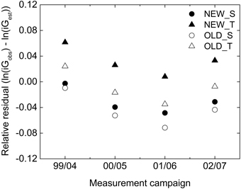
Fig. 2. Average relative residuals for basal area growth by OLD_S (unfilled circle), NEW_S (filled circle), OLD_T (unfilled triangle) and NEW_T (filled triangle) for plots measured in different measurement years in the NFI-data.
The stand-level models had a higher precision than the tree-level models since the standard deviations of the residuals were smaller for the former than for the latter, comparing models calibrated with the same data sets (p < 0.001). The newer models (NEW_S and NEW_T) were also more precise than the older once (OLD_S and OLD_T) (p < 0.001).
Residual trends over different site and stand parameters had mostly similar patterns for the different models (Fig. 3). The overestimation with OLD_S, NEW_S and OLD_T was largest for pine stands, stands with lower site index and stands with lower basal area. For stands with higher basal area all models underestimated the growth. Residuals from NEW_S and OLD_T had opposite trends over age while the overestimation by OLD_S was stable over age.
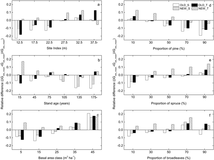
Fig. 3. Difference between average observed and estimated basal area growth (iG, m2 ha–1) over a five year period for the output of the different growth models (OLD_S (unfilled), NEW_S (horizontally hatched), OLD_T (black), NEW_T (obliquely hatched)) relative to observed data from the National Forest Inventory. The residuals are presented for different levels of: (a) the site index (H100), (b) initial total stand age, (c) initial basal area of trees with DBH values above 99 mm, the proportion of the overall basal area that consists of (d) Scots pine, (e) Norway spruce and (f) broadleaved tree species.
3.2 Evaluation of Heureka using GG-data
In average for all plots in the GG-data the basal area growth in the whole observation period was overestimated, for pine at 2.0% by HEU_NEW and at 1.9% by HEU_OLD, for spruce at 3.9% by HEU_NEW and 4.9% by HEU_OLD. There was no clear trend over the prediction period and small differences between treatments (Fig. 4). The standard deviations of the relative residuals did not increase over time. On the contrary they tended to be largest in the first, in average 7-year growth period.
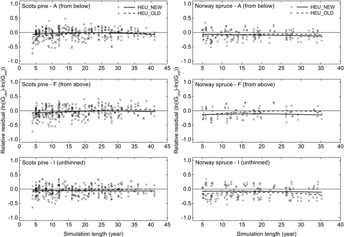
Fig. 4. Relative residuals for the mean annual basal area growth (iG, m2 ha–1 year–1) under different treatments and simulation lengths when comparing the output of Heureka simulations to data from a thinning experiment. Residuals and loess lines for Heureka simulations using HEU_NEW (circle, solid line) and HEU_OLD (cross, dashed line) are shown. Separate calculations were performed for plots of Scots pine and Norway spruce under treatments including light thinning from below (A) and above (F), as well as non-thinned plots (I). For a description of the thinning treatments, see Table 3.
The average predicted volume growth deviated less than 0.5% from that observed for pine and overestimated at about 2.2% for spruce by both HEU_NEW and HEU_OLD. The pattern over time was similar to that for basal area residuals in Fig. 4.
In the variance analysis of relative residuals by HEU_NEW for basal area growth in pine over the whole observation period, a larger overestimation of growth in the non-thinned treatment caused a weak but significant treatment effect. For pine the standard deviation between blocks was greater for HEU_OLD compared to HEU_NEW whereas the opposite was true for spruce (Table 6). The variation in prediction of volume growth was similar to that in basal area growth.
| Table 6. The standard deviations of residuals by HEU_NEW and HEU_OLD (ln(obs)-ln(est)) for basal area and volume growth in the GG-trials over the whole observation period. The variation was split on within and between blocks by variance analyses. There were 40 pine blocks with 4–6 plots per block and 17 spruce blocks with 3–6 plots per block. | ||||||
| Species | Function | Basal area growth | Volume growth | |||
| within | between | within | between | |||
| Pine | HEU_NEW | 0.070 | 0.119 | 0.075 | 0.117 | |
| HEU_OLD | 0.068 | 0.182 | 0.075 | 0.163 | ||
| Spruce | HEU_NEW | 0.101 | 0.156 | 0.098 | 0.180 | |
| HEU_OLD | 0.099 | 0.123 | 0.093 | 0.155 | ||
4 Discussion
First of all it must be stressed that the data used for testing in this study were not totally independent of the data used for model calibration. An earlier measurement period of the NFI-plots used for testing formed a part of the data behind the NEW_T and NEW_S models. The test period was separated from the calibration period by 15 years and most variables, including site index and to a large extent also stand age were estimated independently so we believe that the weak relation between calibration and evaluation data had a minor influence on the results. Selection of plots without mortality means discarding about 15% of the plots. On plots with mortality the growth of dead trees before they died is not included in measured growth. On the other hand the thinning response of remaining trees will give those trees a larger growth than of trees on plots without mortality. In summary we can expect a lower measured growth on plots without than on plots with mortality.
Also data from the thinning experiment was used in model calibration. Early height measurements formed a part of the data behind the site index equations and the density-related adjustment applied at height growth prediction as well as the thinning response models were entirely based on those data. Thus predictions of height and volume growth were highly influenced by the measured development. Still we consider it interesting to include those parts in the study to see how the different components work together in Heureka.
Basal area growth was overestimated at about 2–3% by NEW_S and OLD_T for both NFI-data and GG-data. However, as was shown with NFI-data (Fig. 2) the growth level varies between observation periods so the “true” level is hard to find out in short-term studies. The GG-data was followed over longer periods and can probably reflect the true growth level. An overestimation at 2% by OLD_T could be expected, since that model was based on data from undamaged sample trees. Damaged trees were found to grow 15% less in average, and taking the frequency of damaged trees into account Söderberg (1986) remarked that his models should overestimate the growth at 2%. This remark was overlooked at the programming of Heureka and was thus not considered in our test. Heureka will now be corrected for this. The growth level reflected by NEW_S is less trustworthy since it represents a less underpinned level adjustment of the initial model.
The lower growth level predicted by NEW_T depends on an inaccurate calibration based on year-ring indices. The indices were based on ring-width data in cores from old trees probably disposed to nitrogen fertilization, and so the corresponding index values were unreasonably high (Elfving 2010a). The NEW_S model was based on un-calibrated data and is used for calibration of the stand-level growth in Heureka.
The good agreement between the different growth models is of particular interest. Models based on data from the early 1970s and the late 1980s gave almost accurate predictions for basal area growth in the early 2000s. Also the long-term evaluation indicated a stable growth level over time. Hypothesis 1 was thus not supported. A premise for this result is that age is included as independent variable in the models. It is not possible to measure age of all trees in the forest but the rough system used in Heureka for age estimation seems to be sufficient to stabilize the long-term development.
Empirical growth models are adapted to the information value of the independent variables in calibration data. Age was determined with high precision in the data behind OLD_T but can not be determined at the same precision in most applications. Age determination in NFI is less precise but in line with expectation in normal applications. Thus age is a weaker variable in NEW_S and NEW_T than in OLD_T. Variables describing general growing conditions, to the extent they can be measured, helps to direct the growth prediction in the right direction. This difference between HEU_NEW and HEU_OLD was demonstrated by the spruce data in the thinning experiment. In this data the age was determined with high precision and predictions with HEU_OLD were done with one single model, especially adapted for this population: young spruce (age class) stands in southern Sweden (region). There was also a large growth variation between stands that was poorly reflected by site variables. In this case HEU_OLD had a higher precision than HEU_NEW (Table 6).
All of the growth models tended to underestimate the basal area growth for plots with large initial basal areas. One reason could be border effects on small plots. Plots in denser parts of the stand and close to open areas utilize space outside the plot and vice versa. This effect was however balanced at model construction by special variables expressing density of the plot environment. It is likely that the underestimation is related to the variation in carrying capacity between sites. As was noted by Assman (1961), sites with similar levels of height development as a function of age can have different volume growth. It has not been possible to adequately describe this variation with site variables. The high levels of growth are not attainable in explicitly non-thinned stands, for which growth models generally tends to overestimate the basal area growth, as for the non-thinned plots in the thinning experiment. During the development of the growth models, a conscious decision was taken to limit the positive impact of high initial basal areas in order to avoid biasing results obtained under other conditions; the need to make such compromises is an inherent problem in empirical growth modelling.
It has been argued that stand-level growth models estimate stand-level output more accurately then tree-level models (Qin and Cao 2006; Mäkinen et al. 2008). In a previous study by Härkönen et al. (2010) that used data from NFI plots in Finland to evaluate growth models, tree-level models exhibited a more pronounced tendency to underestimate stand-level basal area growth than did stand-level models. However, the opposite was true for estimates of stand volume growth. An important result of this study is that detailed single tree growth models had lower precision for estimation of total growth than one single stand-based model for all stand types in Sweden. This falsifies our hypothesis 2. It is in line with the so called Occam’s Razor: an efficient model should not be more complicated than necessary to explain the observed variation in a data set. An implication of our finding is that single-tree models could not be expected to give more information on the development of stands with a complex structure (mixed species and ages) than stand-based models. Stand-level and tree-level models gave however sometimes quite different predictions and it is probably possible to increase the precision by making simultaneous parameter estimations for the two model types on basis of the same data-set, as suggested by Yue et al. (2008). The variance analysis on total residuals in the GG-data indicated that the unexplained variation in growth between plots within stands was about 7–10% (standard deviation of relative residuals, Table 6). This variation is hard to explain further since the demands on initial homogeneity of selected plots were large: pure spruce or pine, even-aged, limited variation in basal area and site conditions. The within-stand variation can thus be regarded as a measurement error at the stand level. It can be decreased by increasing the number of measured plots per stand. The pure prediction error, due to unexplained variation in growth between blocks (stands) was in average estimated at around 15%. It did not increase with the length of the prediction period. Hypothesis 3 was thus not supported. Our study did however not include variation caused by random mortality. Larger accidents of high mortality will certainly cause an increased residual variation over time.
Geographic variation was not specifically studied in our evaluation. There were significant residual deviations between counties, both in the basic NFI-data used for model construction and in the NFI-data used for testing. The correlation between the deviations in the two data-sets was, however, weak and it is unclear to what extent those deviations are stable over time. Deeper studies are needed before regional variation can be included in our growth models.
Mortality plays a key role in stand development and is an important component of growth modelling, especially in long-term simulations (Weiskittel et al. 2011). Mortality was not modeled in this work in order to better focus on the accuracy of the growth models per se. However, mortality in the thinning experiment that provided the experimental data used in this work has previously been studied and modeled by Elfving (2010b).
5 Conclusions
Growth models based on historical growth data gave reliable growth predictions up to the century shift, despite the increased growth in our forests. The precision of stand-level growth predictions varied between 0.12–0.18 in the studied experiments and did not decrease with increasing projection period. One single stand-level basal-area growth model for all forests in Sweden performed better than detailed single-tree models for different species. For further improvement, well-designed experiments are needed to explore the stand dynamics in more detail, as a basis for improvement of growth models. Future growth studies should probably focus more on stand-level behavior than on growth of single trees.
Acknowledgements
We would like to thank reviewers for valuable comments on the manuscript. Thanks also to Jan-Eric Englund for statistical consultation. The work was financially supported by the research program Future Forests.
References
Assmann E. (1961). Waldertragskunde. BLV Verlagsgesellschaft, Germany. 490 p. [In German].
Brandel G. (1990). Volymfunktioner för enskilda träd: tall, gran och björk. [Volume functions for indivitual trees: Scots pine (Pinus sylvestris), Norway spruce (Picea abies) and birch (Betula pendula, Betula pubescens)]. Swedish University of Agricultural Sciences, Department of Forest Yield Research, Report 26. 183 p. ISBN 91-576-4030-0. [In Swedish with English summary].
Ekö P.M. (1985). En produktionsmodell för skog i Sverige, baserad på bestånd från riksskogstaxeringens provytor. [A growth simulator for Swedish forests, based on data from the national forest survey]. Swedish University of Agricultural Sciences, Department of Silviculture, Report 16. 224 p. ISBN 91-576-2386-4. [In Swedish with English summary].
Elfving B. (2003). Ålderstilldelning till enskilda träd i skogliga tillväxtprognoser. [Estimation of age of single trees in forest yield forecasts]. Swedish University of Agricultural Sciences, Department of Silviculture, Working Paper 182. 44 p. [In Swedish].
Elfving B. (2010a). Growth modelling in the Heureka system. Swedish University of Agricultural Sciences, Faculty of Forestry. http://heurekaslu.org/wiki/Heureka_prognossystem_(Elfving_rapportutkast).pdf. [Cited 17 March 2014]
Elfving B. (2010b). Natural mortality in thinning and fertilization experiments with pine and spruce in Sweden. Forest Ecology and Management 260(3): 353–360. http://dx.doi.org/10.1016/j.foreco.2010.04.025.
Elfving B., Kiviste A. (1997). Construction of site index equations for Pinus sylvestris L. using permanent plot data in Sweden. Forest Ecology and Management 98: 125–134. http://dx.doi.org/10.1016/S0378-1127(97)00077-7.
Elfving B., Tegnhammar L. (1996). Trends of tree growth in Swedish forests 1953–1992: an analysis based on simple trees from the National Forest Inventory. Scandinavian Journal of Forest Research 11: 26–37. http://dx.doi.org/10.1080/02827589609382909.
Hägglund B. (1981). Forecasting growth and yield in established forests. Swedish University of Agricultural Sciences, Department of Forest Survey, Report 31. 145 p. ISBN 91-576-0797-4.
Hägglund B., Lundmark J.-E. (1977). Site index estimation by means of site properties. Studia Forestalia Suecica 138. 38 p.
Härkönen S., Mäkinen A., Tokola T., Rasinmäki J., Kalliovirta J. (2010). Evaluation of forest growth simulators with NFI permanent sample plot data from Finland. Forest Ecology and Management 259: 573–582. http://dx.doi.org/10.1016/j.foreco.2009.11.015.
Holm S. (1981). Analys av metoder för tillväxtprognoser i samband med långsiktiga avverkningsberäkningar. Swedish University of Agricultural Sciences, Department of Biometry and Forest Management, Working Paper. 22 p. [In Swedish].
Kangas A.S. (1997). On the prediction bias and variance in long-term growth projections. Forest Ecology and Management 96: 207–216. http://dx.doi.org/10.1016/S0378-1127(97)00056-X.
Mäkinen A., Kangas A., Kalliovirta J., Rasinmäki J., Välimäki E. (2008). Comparison of treewise and standwise forest simulators by means of quantile regression. Forest Ecology and Management 255: 2709–2717. http://dx.doi.org/10.1016/j.foreco.2008.01.048.
Näslund M. (1936). Skogsförsöksanstaltens gallringsförsök i tallskog. Meddelanden från Statens skogsförsöksanstalt 29. 169 p. [In Swedish with English summary].
Nilsson U., Agestam E., Ekö P.M., Elfving B., Fahlvik N., Johansson U., Karlsson K., Lundmark T., Wallentin C. (2010). Thinning of Scots pine and Norway spruce monocultures in Sweden – effects of different thinning programmes on stand level gross- and net stem volume production. Studia Forestalia Suecica 219. 46 p.
Pettersson H. (1955). Barrskogens volymproduktion. Meddelanden från Statens skogsforsknings-institut 45. 391 p. [In Swedish].
Pretzsch H., Biber P., Ďurský J. (2002). The single tree-based stand simulator SILVA: construction, application and evaluation. Forest Ecology and Management 162: 3–21. http://dx.doi.org/10.1016/S0378-1127(02)00047-6.
Qin J., Cao Q.V. (2006). Using disaggregation to link individual-tree and whole-stand growth models. Canadian Journal of Forest Research 36: 953–960. http://dx.doi.org/10.1139/x05-284.
Ranneby B., Cruse T., Hägglund B., Jonasson H., Swärd J. (1987). Designing a new national forest survey for Sweden. Studia Forestalia Suecica 177. 29 p.
Söderberg U. (1986). Funktioner för skogliga produktionsprognoser: tillväxt och formhöjd för enskilda träd av inhemska trädslag i Sverige. [Functions for forecasting of timber yields: increment and form height for individual trees of native species in Sweden]. Swedish University of Agricultural Sciences, Section of Forest Mensuration and Management, Report 14. 251 p. ISBN 91-576-2634-0. [In Swedish with English summary].
Söderberg U., Ranneby B., Chuanzhong L. (1993). A diameter growth index method for standardization of forest data inventoried at different dates. Scandinavian Journal of Forest Research 8: 418–425. http://dx.doi.org/10.1080/02827589309382788.
Svensson S.A. (1980). The Swedish National Forest Survey, 1973–1977: state of forests, growth and annual cut. Swedish University of Agricultural Sciences, Department of Forest Survey, Report 30. 167 p. ISBN 91-576-0681-1. [In Swedish with English summary].
Teuffel K., Hein S., Kotar M., Preuhsler E.P., Puumalainen J., Weinfurter P. (2006). End user needs and requirements. In: Hasenauer H. (ed.). Sustainable forest management – growth models for Europe. Springer Berlin Heidelberg, Germany. p. 19–38. http://dx.doi.org/10.1007/3-540-31304-4_2.
Valinger E. (1992). Effects of thinning and nitrogen fertilization on stem growth and stem form of Pinus sylvestris trees. Scandinavian Journal of Forest Research 7: 219–228. http://dx.doi.org/10.1080/02827589209382714.
Vanclay J.K., Skovsgaard J.P. (1997). Evaluating forest growth models. Ecological Modelling 98: 1–12. http://dx.doi.org/10.1016/S0304-3800(96)01932-1.
Weiskittel A.R., Hann D.W., Kershaw J.A., Vanclay J.K. (2011). Forest growth and yield modelling. John Wiley and Sons Ltd, Chichester, West Sussex, UK. http://dx.doi.org/10.1002/9781119998518.
Wikström P., Edenius L., Elfving B., Eriksson L.O., Lämås T., Sonesson J., Öhman K., Wallerman J., Waller C., Klintebäck F. (2011). The Heureka forestry decision support system: an overview. Mathematical and Computational Forestry and Natural-Resource Sciences 3(2): 87–94.
Yue C., Kohnle U., Hein S. (2008). Combining tree- and stand level models: a new approach to growth prediction. Forest Science 54(5): 553–566.
Total of 29 references
