Ana de Lera Garrido  ,
Terje Gobakken,
Hans Ole Ørka,
Erik Næsset,
Ole M. Bollandsås
,
Terje Gobakken,
Hans Ole Ørka,
Erik Næsset,
Ole M. Bollandsås
Reuse of field data in ALS-assisted forest inventory
de Lera Garrido A., Gobakken T., Ørka H. O., Næsset E., Bollandsås O. M. (2020). Reuse of field data in ALS-assisted forest inventory. Silva Fennica vol. 54 no. 5 article id 10272. https://doi.org/10.14214/sf.10272
Highlights
- Six biophysical forest attributes were estimated for small stands without using up-to-date field data
- The approaches included reused model relationships and forecasted field data
- The accuracy of height estimates was comparable with the accuracy of an ordinary forest inventory with up-to-date field- and ALS data
- Both approaches tended to produce estimates systematically different from the ground reference.
Abstract
Forest inventories assisted by wall-to-wall airborne laser scanning (ALS), have become common practice in many countries. One major cost component in these inventories is the measurement of field sample plots used for constructing models relating biophysical forest attributes to metrics derived from ALS data. In areas where ALS-assisted forest inventories are planned, and in which the previous inventories were performed with the same method, reusing previously acquired field data can potentially reduce costs, either by (1) temporally transferring previously constructed models or (2) projecting field reference data using growth models that can serve as field reference data for model construction with up-to-date ALS data. In this study, we analyzed these two approaches of reusing field data acquired 15 years prior to the current ALS acquisition to estimate six up-to-date forest attributes (dominant tree height, mean tree height, stem number, stand basal area, volume, and aboveground biomass). Both approaches were evaluated within small stands with sizes of approximately 0.37 ha, assessing differences between estimates and ground reference values. The estimates were also compared to results from an up-to-date forest inventory relying on concurrent field- and ALS data. The results showed that even though the reuse of historical information has some potential and could be beneficial for forest inventories, systematic errors may appear prominent and need to be overcome to use it operationally. Our study showed systematic trends towards the overestimation of lower-range ground references and underestimation of the upper-range ground references.
Keywords
airborne laser scanning;
data reuse;
temporal model transferability
-
de Lera Garrido,
Faculty of Environmental Sciences and Natural Resource Management, Norwegian University of Life Sciences, P.O. Box 5003, NO-1432 Ås, Norway
E-mail
ana.maria.lera.garrido@nmbu.no
- Gobakken, Faculty of Environmental Sciences and Natural Resource Management, Norwegian University of Life Sciences, P.O. Box 5003, NO-1432 Ås, Norway E-mail terje.gobakken@nmbu.no
- Ørka, Faculty of Environmental Sciences and Natural Resource Management, Norwegian University of Life Sciences, P.O. Box 5003, NO-1432 Ås, Norway E-mail hans-ole.orka@nmbu.no
- Næsset, Faculty of Environmental Sciences and Natural Resource Management, Norwegian University of Life Sciences, P.O. Box 5003, NO-1432 Ås, Norway E-mail erik.naesset@nmbu.no
- Bollandsås, Faculty of Environmental Sciences and Natural Resource Management, Norwegian University of Life Sciences, P.O. Box 5003, NO-1432 Ås, Norway E-mail ole.martin.bollandsas@nmbu.no
Received 18 November 2019 Accepted 22 September 2020 Published 23 October 2020
Views 87599
Available at https://doi.org/10.14214/sf.10272 | Download PDF

1 Introduction
Forest management inventories (FMI) assisted by airborne laser scanning (ALS) have been conducted operationally since 2002 (Næsset 2014). The reliability of estimates of biophysical forest attributes (BFA) such as dominant height, stand basal area, volume, or aboveground biomass using ALS, has been demonstrated in several studies (Næsset 2004c; Hyyppä et al. 2008; Woods et al. 2011). However, the efficiency of an inventory depends on the inventory costs as well as the accuracy and precision of the estimates.
In the planning process of ALS inventories, several decisions affecting costs have to be made (Maltamo et al. 2011; Næsset 2014), both related to the ALS acquisition and the field inventory, which also affect the precision and accuracy of the BFA estimates. Furthermore, there are costs associated with incorrect management decisions caused by erroneous inventory information (Eid et al. 2004; Kangas et al. 2018). The difference in economic return between the potential optimal decision and the actual sub-optimal decision is the cost in this case. Thus, the decisions regarding ALS acquisitions and field inventory should be made after careful considerations of both the expected costs and accuracy of the resulting forest information. The cost of sub-optimal decisions can be determined using cost-plus-loss analyses (Hamilton 1978), where the expected costs and returns of a scenario with perfect inventory information, are compared to the cost and returns of a scenario with errors in the inventory information. Using such analysis, Eid et al. (2004) showed that BFA estimates from ALS inventories may result in less erroneous management decisions and smaller total costs than inventory methods based on photointerpretation.
Maltamo et al. (2011) analyzed the effects of different plot selection strategies associated with ALS-assisted inventories and listed several measures to reduce costs. The listed measures are related to the choice of modeling technique, ALS acquisition parameter settings, and reduced field efforts such as reduced sampling intensities or reuse of existing data. In this context, reuse data means to use existing co-registered field- and ALS data from a previous inventory to construct predictive models that can be transferred in time and applied to the area of interest (AOI) with current ALS data, without measuring new field plots. Models could also be spatially transferred between AOIs. Furthermore, previously measured field data could be utilized without concurrent ALS data if they are projected to the time of the ALS acquisition using models of forest dynamics.
Temporally and spatially transferred models have been applied in many fields, such as transport planning (Fox et al. 2014), hydrology (Li et al. 2012), and ecology (Barbosa et al. 2009; Rapacciuolo et al. 2012; Yates et al. 2018) to support management decisions in cases where resources for collecting up-to-date data are limited. In the context of ALS forest inventories, a few studies have been conducted transferring regression models spatially (Foody et al. 2003; Næsset and Gobakken 2008; Kotivuori et al. 2018; Tompalski et al. 2019) or temporally (Fekety et al. 2015; Hou et al. 2017; Zhao et al. 2018; Domingo et al. 2019) with good results. However, transferring models assumes that similar relationships exist between field and ALS data for the different AOIs or the different points in time.
Norway was the first country to use ALS data operationally for FMI. Starting in 2017, those areas inventoried from 2002 and onwards have been subject to the second cycle of ALS data acquisition. Studies of the benefits and challenges related to reusing or projecting field measurements from previous inventories are therefore timely. Reuse of data from the first cycle of inventories could not only reduce the costs of new inventories but also add extra value to the previous information, increasing the profitability of the initial investment.
In the current study, we tested two approaches that reused historical data from an ALS-assisted FMI without up-to-date field information; (1) the reuse of historical information through temporal model transfer (REUSE approach) and (2) the projection of historical field plot information to serve as field reference data for construction of ALS-to-field models with up-to-date ALS data (FORECAST approach).
The objective of this study was to assess the prediction accuracy of estimated BFA under the assumption of unavailable up-to-date field measurements combined with current ALS data. We constructed models for the relationship between field reference data and ALS metrics according to the two approaches mentioned above and applied the models to small forest stands. Both approaches were evaluated by assessing the differences between BFA and corresponding field reference data of the small stands. Moreover, both approaches were compared to results from a conventional ALS forest inventory relying on concurrent field and ALS data (NEW approach).
2 Material and methods
2.1 Study area and stand delineation
The study was conducted in the municipality of Krødsherad (60°10´N, 09°35´E, 130–660 m above sea level) in southeastern Norway (Fig. 1). The dominant tree species in this area are Norway spruce (Picea abies (L.) Karst.) and Scots pine (Pinus sylvestris L.), with large proportions of deciduous species in some parts, mainly birch (Betula pubescens Ehrh.).
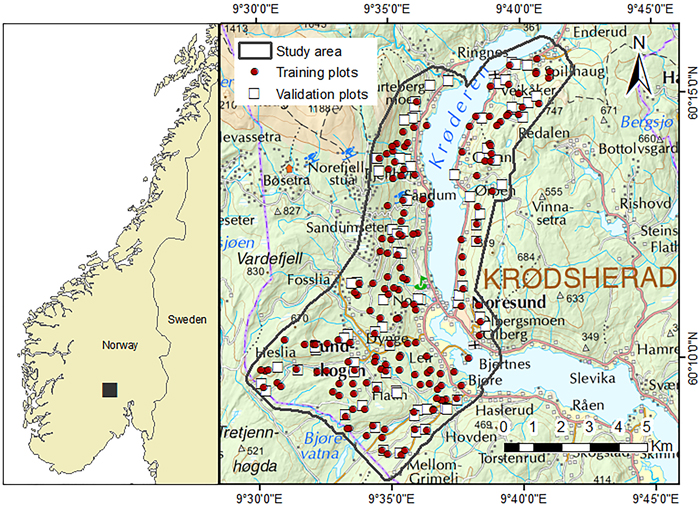
Fig. 1. Map of the location of the study area and field plot positions.
Following the same procedure as in Næsset (2004b), the stands were manually delineated and stratified based on photointerpretation into three different strata according to site productivity, represented by an age-height site index (SI) with an index age of 40 years (Tveite 1977; Tveite and Braastad 1981), and a national system of maturity classification (Eid 2001). These stratification criteria have proven expedient in many studies relating BFAs to ALS metrics, and they are also applied in operational forest inventories in Norway. We excluded stands in the regeneration phase according to the maturity classification system (dominant height < ~8 m) or if deciduous species were dominant. The remaining stands were classified according to the maturity classification system as either “young” (dominant height < ~14 m) or “mature” (dominant height > ~14 m). The stands defined as “young” were all assigned to Stratum 1. The mature stands were assigned to two mutually exclusive strata according to SI. Stratum 2 comprised mature forest with SI ≤ 11 m and Stratum 3 comprised mature forest with SI > 11 m.
2.2 Field data
In the current study, we worked with two different types of plots: training plots used for model construction and validation plots used for independent model validation. Field data for both types of plots were initially registered during the summer of 2001 (T1), and later during the summers of 2016 and 2017 (T2), both times as part of operational forest inventories.
The training plots were circular with an area of 232.9 m2. At T1, they were distributed systematically across each stratum according to independent sampling grids for the respective strata. There were approximately 40 plots per stratum.
The validation plots, that constituted our target population, were planned to be squares with dimensions 61 m × 61 m, which corresponds to the accumulated area of 16 training plots. However, due to some practical difficulties when the validation plot corners were established in field, their final sizes and shapes varied. They were located at T1 in subjectively selected stands covering a wide range of forest conditions within the strata they represented. However, in the current study we excluded validation plots that were partially harvested in the period between T1 and T2, covered more than a single stratum at T2.
Planimetric coordinates of training plot centers and validation plot corners were registered by means of differential global navigation satellite systems (GNSS) at T1 and marked with wooden sticks, and at T2 real time kinematic GNSS navigation was used to navigate to the original positions. The positions were remeasured using differential GNSS for those training plot centers and validation plot corner where the wooden stick from T1 could not be found.
2.3 Field measurements and calculation of BFAs
For the trees within each training plot, diameter at breast height (dbh) was callipered. For the young (Stratum 1) and mature forest (Strata 2 and 3), the lower diameter limits were 4 cm and 10 cm, respectively. Among the callipered trees, sample trees for height measurements were selected proportional to stem basal area using a relascope. The basal area factor (Bitterlich 1984) was selected for each sample plot so that approximately 10 sample trees would be selected in each plot. On plots with fewer than 10 trees, all trees were selected as sample trees (Næsset 2004b). For the validation plots, sample trees were also selected proportional to stem basal area by applying sampling fractions (every n’th calliper tree) determined specifically to each diameter class. Fifty-eight trees were selected on average for each validation plot.
Stem number was computed as number of trees per hectare (N) based on the callipered trees. Accordingly, stand basal area (G) was computed as basal area per hectare of the callipered trees. Since only a sample of the trees were measured for height, total plot volume (V) and aboveground biomass (AGB) were calculated using a ratio estimator as described in Ørka et al. (2018). Furthermore, we predicted the height of each tree using the volume models (Braastad 1966; Brantseg 1967; Vestjordet 1967), setting the height as unknown. From the predicted heights, dominant height (Ho) was calculated for each plot as the mean height of the two largest trees according to dbh. Plot-level mean height (HL), was computed as the basal area-weighted mean height (Lorey’s mean height). Table 1 shows a summary of ground reference data by stratum.
| Table 1. Summary of the ground reference biophysical forest attributes by stratum (after season correction). | ||||||||
| Young forest | Mature forest SI ≤ 11 m | Mature forest SI > 11 m | ||||||
| Range | mean | Range | mean | Range | mean | |||
| Training plots | 2001 | n | 35 | 37 | 37 | |||
| Ho | 10.3–25.1 | 17.6 | 10.7–25.5 | 17.5 | 18.8–28.9 | 23.4 | ||
| HL | 8.2–20.5 | 13.8 | 9.9–23.5 | 15.7 | 15.8–26.8 | 20.6 | ||
| N | 386–3693 | 1809 | 172–1632 | 629 | 301–1503 | 819 | ||
| G | 6.4–62.6 | 25.1 | 5.3–43.1 | 22.7 | 15.5–56.9 | 34.2 | ||
| V | 29.8–642.9 | 187.8 | 28.7–420.3 | 178.9 | 121.2–681.6 | 337.5 | ||
| AGB | 19.1–368.6 | 117.2 | 17.7–241.6 | 102.9 | 76.6–355.0 | 192.9 | ||
| 2016 | n | 40 | 34 | 42 | ||||
| Ho | 11.9–28.8 | 18.2 | 11.5–25.7 | 18.2 | 17.5–30.3 | 22.9 | ||
| HL | 9.0–25.2 | 14.9 | 11.0–24.3 | 16.6 | 14.8–25.9 | 19.8 | ||
| N | 429–3220 | 1545 | 129–1331 | 609 | 301–3521 | 958 | ||
| G | 6.2–72.6 | 27.9 | 5.3–58.4 | 26.6 | 14.2–72.2 | 34.6 | ||
| V | 26.4–904.3 | 214.6 | 30.3–532.6 | 220.9 | 100.9–819.2 | 328.6 | ||
| AGB | 20.3–499.7 | 136.5 | 19.0–286.2 | 127.1 | 73.6–404.1 | 185.3 | ||
| Forecasted 2016 | n | 12 | 33 | 42 | ||||
| Ho | 14.0–27.2 | 18.9 | 11.8–26. 5 | 18.5 | 15.9–30 .0 | 22.1 | ||
| HL | 11.6–22.9 | 15.7 | 11.0–24.4 | 16.9 | 13.0–28.0 | 19.2 | ||
| N | 429–2319 | 1417 | 172–1202 | 599 | 301–3306 | 1114 | ||
| G | 15.8–86.8 | 34.8 | 7.4–60.1 | 28.4 | 12.7–73.3 | 38.9 | ||
| V | 97.7–975.2 | 292.2 | 41.9–582.5 | 237.0 | 104.1–903.3 | 357.6 | ||
| AGB | 62.0–552.3 | 178.4 | 26.1–311.8 | 135.6 | 73.5–439.8 | 204.0 | ||
| Validation plots | 2016 | n | 11 | 14 | 24 | |||
| Ho | 16.1–20.7 | 18.3 | 13.7–24.6 | 17.9 | 17.6–26.4 | 23.1 | ||
| HL | 13.5–17.2 | 15.4 | 12.1–20.9 | 15.9 | 14.9–25.1 | 20.4 | ||
| N | 452–1712 | 1254 | 201–1147 | 632 | 337–1221 | 762 | ||
| G | 13.9–30.7 | 25.7 | 10.4–40.8 | 22.9 | 17.9–46.5 | 30.6 | ||
| V | 99.1–241.6 | 194.1 | 68.8–359.8 | 178.6 | 124.5–525.2 | 298.7 | ||
| AGB | 64.6–163.0 | 125.7 | 41.2–221.1 | 108.6 | 87.2–294.8 | 170.0 | ||
| SI = site index, n = Number of plots. Biophysical forest attributes: Ho = Dominant height (m), HL = Lorey’s mean height (m), N = Stem number (ha–1), G = Basal area (m2 ha–1), V = Volume (m3 ha–1), AGB = Aboveground biomass (Mg ha–1). | ||||||||
2.3.1 Correction within growth season
ALS and field data were acquired at different dates, either within the same growth season or between adjacent growth seasons. Therefore, the field values were adjusted using growth models to match the date of the ALS acquisition. All BFAs, except N, were corrected. We assumed the growth to be nonlinear relative to the progress of the number of days into the growing season.
Based on data from an official weather station 10 km from the center of the study area, the growth season start date was estimated as the mean day-number when the degree-day sum exceeded 10 °C in the period between 2001 and 2016 (day 125). We assumed that the tree height growth season was 60 days long (Sharma et al. 2011). For the rest of the BFAs, the growth season end date was set to day 230 (Mäkinen et al. 2008).
For each BFA, a corrected value was calculated as:
![]()
where SG is the season growth, calculated as the difference between the value of the biophysical forest attribute at T2 and T1, divided by the number of growth seasons in between. CP is the correction period, corresponding to the relative progress into the growth season at the date of the ALS acquisition minus the relative progress into the growth season at the date of field measurements (Sharma et al. 2011). CP values can be either positive or negative, depending on whether the field data were acquired before or after the ALS data.
2.4 Airborne laser scanning
ALS data were collected under leaf-on conditions by fixed-wing aircrafts, using different ALS instruments at each point in time. Using standard procedures, the contractors undertook complete post processing of the three-dimensional clouds of echoes, performing the filtering, classification of ground- and vegetation echoes, and normalization. At T1 and T2, Optech ALTM 1210 and Riegl LMS Q-1560 sensors were used, respectively. The Riegl sensor can record multiple echoes from each pulse. In the current study, we used only “first”, “last” and “single” echoes. However, “single” echoes were pooled together with “first” when constructing the ALS-metrics (see below). The respective data acquisition parameters are shown in Table 2.
| Table 2. Airborne laser scanning acquisition parameters. | ||
| Year of acquisition | 2001 (T1) | 2016 (T2) |
| Time period | 23 June – 1 August | 7 June – 31 July |
| Aircraft | Piper PA-31 | Piper PA-31 |
| Laser scanning system | Optech ALTM 1210 | Riegl LMS Q-1560 |
| Operating firm | Fotonor AS | Terratec AS |
| Average flying altitude (m) | 650 | 1280 |
| Average flying speed (m s–1) | 75 | 69 |
| Pulse repetition frequency PRF (kHz) | 10 | 534 |
| Scanning frequency (kHz) | 30 | 115 |
| Side overlap (%) | 50 | 20 |
| Maximum scan angle (degrees) | 15 | 20 |
| Average point density (pts m–2) | 0.9 | 11.8 |
2.4.1 ALS metrics
For each plot, height- and canopy density metrics for first and last echoes were computed from the clouds of echoes from each point in time.
Height-related variables including maximum value (Hmax), mean value (Hmean), coefficient of variation (Hcv), standard deviation (Hsd), and heights at percentiles of 10% intervals (H10, H20, …, H90) were computed from the laser echo height distributions, excluding echoes < 2 m to eliminate falsely classified echoes close to the ground and the effect of boulders, low vegetation, etc. (Nilsson 1996). When calculating canopy density metrics, we divided the height range between the 2 m threshold and the 95th height percentile into ten bins of equal length, and then density metrics (D0, D1, …, D9) were calculated as the proportion of echoes above the lower limit of each bin and the total number of echoes including those below the threshold of 2 m (Gobakken and Næsset 2008). For all variables, the suffixes “.F”, “.L” specified whether the metrics were computed from the height distributions of first or last laser echoes.
2.5 Projection of biophysical forest attributes to T2
On the training plots, we applied species-specific, individual tree, growth models to project diameter (Bollandsås et al. 2008) and height (Sharma and Brunner 2017) of single trees from T1 to the date of the ALS acquisition at T2. We also applied models predicting individual tree mortality (Eid and Tuhus 2001) during the observation period. With these forecasted values we calculated new field values for all the BFA (Fig. 2 FORECAST) following the method described in section 2.3, but without applying the season correction. A summary of the forecasted field values by strata is displayed in Table 1 (Forecasted 2016).
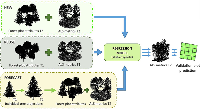
Fig. 2. Conceptual framework of the three approaches. Top: The NEW approach represents concurrent ALS and field reference values from T2 used to construct models that later were used to make predictions on the validation plots. Middle: The REUSE approach applies temporally transferred models from T1 to predict the forest attributes at T2. Bottom: The FORECAST approach applies data projected from T1 to T2 together with ALS data from T2 used to construct models that were used for predictions on the validation plots.
2.6 Model construction
We developed stratum-specific models for the six BFAs. During preliminary analyses, it was observed that not all BFAs were linearly related to the ALS metrics, and therefore we constructed nonlinear models with an automated variable selection procedure as described in Ørka et al. (2016). The variable selection entails a first step for constructing linear models with logarithmically transformed variables with an exhaustive search using the stepwise algorithm ‘regsubsets’ from the leaps package (Lumley 2004) in R. The best models were selected among those including up to three explanatory variables based on the Bayesian information criterion (BIC) and the Variance inflation factor (VIF < 5). Finally, nonlinear models (Eq. 2) were constructed with the selected explanatory variables on the original scale using the ‘nls’ function in R, with the Gauss-Newton algorithm. We used the parameter estimates of the corresponding linear regression model, transformed to arithmetic scale, as starting values.
![]()
where y is the response variable, a, b, and c are the potential explanatory variables, β0, β1, β2 and β3 are the parameters to be estimated and ε is the error term.
2.6.1 Approaches
Using the methodology explained above, we constructed stratum-specific models for three approaches, designated NEW, REUSE, and FORECAST.
With the NEW approach, models were constructed with the data from the training plots measured at T2 (Fig. 2). These models represent a conventional ALS forest inventory based on up-to-date data, and the results were used as benchmarks for the two other approaches.
With the REUSE approach, we constructed models with the data from the training plots at T1. The models were used for prediction with ALS metrics from T2 (Fig. 2). Thus, this approach addressed temporal model transferability.
With the FORECAST approach, T1 measurements were forecasted to the date of the ALS acquisition at T2. Then, stratum-specific models for the forecasted BFA dependent on ALS metrics from T2 were constructed (Fig. 2). Most of the plots classified as young at T1 evolved to mature forest after projection, and only 12 plots remained in Stratum 1. We considered this to be an insufficient number of plots for model construction. Therefore, models for this stratum were based on the entire projected training plot dataset.
2.7 Model fit
The fit of all models was assessed by the pseudo-R2 (r2), calculated as one minus the ratio between the residual sum of squares and the total sum of squares. We also calculated the root mean square error relative to the ground reference values (RMSE%) as
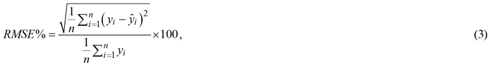
where n is the number of plots, ![]() is the ground reference value for plot i, and
is the ground reference value for plot i, and ![]() is the model-fitted value for plot i. However, RMSE has some limitations with regard to disentangling the different components of the uncertainties, making the interpretation difficult (Wallenius et al. 2012). Therefore, to describe and quantify more concisely the error structures, we constructed error models for the fitted values
is the model-fitted value for plot i. However, RMSE has some limitations with regard to disentangling the different components of the uncertainties, making the interpretation difficult (Wallenius et al. 2012). Therefore, to describe and quantify more concisely the error structures, we constructed error models for the fitted values ![]() with the ground reference values
with the ground reference values ![]() as explanatory information, as described in Persson and Ståhl (2020). The model (Eq. 4) was a linear model fitted with ordinary least squares method and the three parameters λ0, λ1, and σε, were used to interpret the error structure:
as explanatory information, as described in Persson and Ståhl (2020). The model (Eq. 4) was a linear model fitted with ordinary least squares method and the three parameters λ0, λ1, and σε, were used to interpret the error structure:
![]()
The parameters of the model can in this context be interpreted as different components of the model error. λ0 represents the constant systematic displacement of the fitted values, λ1 represents how the systematic error varies across the range of ground reference values, and εem represents the random error. The standard deviation of the random error ![]() represents the size of the unexplained random variation.
represents the size of the unexplained random variation.
2.8 Validation
The validation plots were divided into 16 prediction cells and ALS metrics were calculated for each cell. All models were applied to the prediction cells, and BFAs were estimated for each validation plot as the mean over the respective cell predictions. However, when the mean values were estimated, a weighting was performed for the various BFAs. For N, G, V, and AGB the mean values were estimated by using the area of the respective prediction cells as weights. For Ho and HL the number of ALS echoes > 2 m were used as weights. We calculated the mean prediction difference (MPD) between estimated and ground reference values and tested if they were significantly different from zero using a t-test. As for the model fit, we also calculated the RMSE% and constructed error models. For the validation, Eq. 3 and Eq. 4 applies, but the model fitted values must be substituted with the predicted values. Finally, we applied t-tests for the hypotheses λ0 = 0and λ1 = 1.
For visualization of the error structure and the λ-parameters, density plots of the distributions of the ground reference values and the different estimated values were plotted for all the BFAs, strata, and approaches (Fig. 3). In these density plots, a λ0 ≠ 0will be visible as a shift of the distributions for estimated values in comparison with the corresponding ground references. A λ1 ≠ 1 will be manifested through differing ranges between the distributions of estimates and ground references.
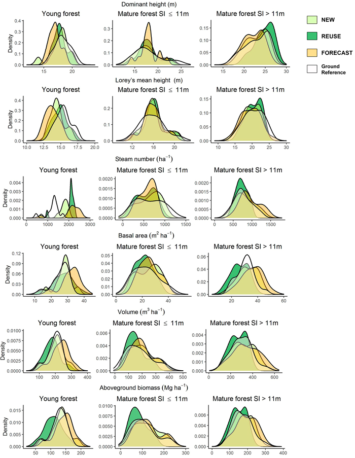
Fig. 3. Density plots showing the distributions of the ground references and the estimated biophysical forest attributes for the different approaches.
3 Results
3.1 Modeling of BFAs
The selected explanatory variables and fit of the regression models are shown in Table 3. The results from the error modeling indicated that none of the models yielded fitted values free from systematic errors (λ0 ≠ 0and λ1 ≠ 1). In cases where λ0 > 0, values of λ1 < 1 implies that fitted values in the lower range of the ground references have positive errors, and values in the upper range have negative. Our results showed that RMSE% were largest for the models for N, they also obtained the smallest r2 and λ1-values. Models for Ho and HL scored highest on the model evaluation criteria, with the largest r2, smallest RMSE% values, and λ1 close to 1.
| Table 3. Selected variables for the predictive nonlinear models of biophysical forest attributes (BFA) by approach and their respective model fit and error structure. View in new window/tab. |
In general, models constructed with the REUSE and NEW approaches, based on contemporary field and ALS data, seemed to deviate less to the calibration data compared to the FORECAST approach. More specifically, in Stratum 1 the models developed with the REUSE approach had the smallest RMSE%. The error modeling showed that the models for G, V, and AGB constructed with the forecasted data resulted in larger values of λ0 and values of λ1 further away from the value of 1, compared to those models constructed with the NEW approach. However, for the modeled heights (Ho and HL), the results were in favor of the FORECAST compared to the NEW approach. In Stratum 2, the smallest RMSE% values were obtained with the NEW approach, followed by REUSE and FORECAST. However, the error modeling showed that the NEW models always resulted in the largest values of λ0. In Stratum 3, models constructed with the FORECAST approach seemed to be adequate judged by the RMSE% and the error modeling. For the REUSE approach in this stratum, values of λ0 were larger, and values of λ1 were further away from the value of 1, compared to the other approaches.
3.2 Estimation of BFAs on validation plots
Table 4 shows the results of the estimation for the large validation plots. In general, the NEW approach yielded the smallest RMSE% values ranging between 4% (Ho) and 38% (N). RMSE%-values for the FORECAST approach were the largest, ranging between 4% (Ho) and 73% (N). Furthermore, there were MPD-values significantly different from zero with all approaches, but especially with the FORECAST approach.
| Table 4. Validation accuracy assessment of the biophysical forest attributes (BFA) estimates. View in new window/tab. |
The error modeling showed that there were statistically significant trends in the estimation deviations for each of the approaches. However, in the NEW approach with contemporary training and estimation data, the trends (λ1 ≠ 1) were statistically significant only for Ho in Strata 2 and 3, N in Stratum 2, and HL in Stratum 3. The results for Stratum 1 were adequate for all approaches with a couple of exceptions. In Stratum 2, however, systematic deviations of the estimates were obtained using both the REUSE and the FORECAST approach. The results indicated a general deviation (λ0 ≠ 0) and a trend towards overestimating plots with small ground reference values of the BFAs and underestimating the upper range of the BFA. The same trends were apparent also in Stratum 3, but not to the same degree as in Stratum 2.
Fig. 3 indicates that the range of the distributions of estimates most often tends to be narrower than the ground references distributions, which corresponds to λ1 < 1. It can also be seen that the FORECAST approach has distributions most frequently shifted outside those from the other approaches.
4 Discussion
This study focused on the analysis of two approaches for reusing field data compared to area-based ALS-assisted forest inventory. Our results suggest that even though reuse of historical information has potential and could be beneficial for forest inventories, there are limitations in the application of either the reused model relationships or the forecasted field data, which will be discussed below.
4.1 Modeling of BFAs
As can be seen from the modeling results (Table 3), the model fits were comparable to other studies on modeling BFAs from ALS metrics (Næsset 2007). However, the distribution of fitted values had a narrower range than the ground reference values in the training data (λ1 < 1). This effect is known as “regression dilution” or “regression towards the mean” (Fuller 2009). It originates from errors in the explanatory variables which are not accounted for in the model fitting when sum of the squared differences between observations of the dependent variable and the fitted model is minimized in the Y direction. To overcome this limitation, and when errors in both X and Y are assumed to be known, total least squares can be applied. Deming regression is one such regression technique, and uses the ratio between the error variance of X and the error variance of Y to adjust the direction that is minimized, yielding a steeper regression line (Fuller 2009). However, there are two drawbacks with this modeling approach. The first and already mentioned is that the true error variance is often not known. Second, it is only two-dimensional. Therefore, models with multiple explanatory variables cannot be fitted.
In preliminary analyses in the current study, we fitted models using Deming regression with a single principal component composed as a linear combination of all available explanatory variables, and with the sample variances of X and Y as proxies for the true error variances. A validation showed that the models fitted with nonlinear least squares mostly outperformed the Deming models judged by MPD, RMSE%, and the error modeling, and the results were thus not reported. Even though the deviations were quite uniformly distributed over the range of the ground reference values, at least for the NEW approach (Table 4), the use of Deming regression should be investigated further if reliable estimates of the true error variances of both X and Y are available.
4.2 Estimation of BFAs on validation plots
In general, the NEW approach that relied on up-to-date field measurements with concurrent ALS data produced more accurate and precise estimates compared to the other approaches. The results of the NEW approach are in accordance with previous studies in the same area that used concurrent field and ALS data to predict plot BFA (Næsset 2004b; Næsset 2007; Gobakken et al. 2012).
The height estimates obtained using the REUSE approach were similar to those obtained using the NEW approach in terms of RMSE% and were also consistent with Tompalski et al. (2019). HL seemed to be the most robust BFA with respect to temporal model transfer. However, for the remaining BFAs, the values of RMSE% were larger. The error modeling also showed systematic deviances that depended on the size of the ground reference value, especially for the two mature strata. This could be attributed to the different sensors and acquisition parameters used at the two points in time, which could affect the properties of the cloud of echoes under otherwise equal conditions (Næsset 2004a; Næsset 2009) and hence also the derived metrics. Although Tompalski et al. (2019) conclude that the robustness of model transfer is more related to the attribute that is being predicted and the modeling approach, changed functional relationships between the ALS metrics and the BFAs are bound to affect the accuracy and precision of the estimates (Hou et al. 2017).
Fekety et al. (2015) combined ALS data collected with Leica sensors at both points in time with a large difference in echo densities (on the order of 1:30). They concluded that even such a great density difference did not affect model transferability. However, in an operational inventory without control data registered in field, it is impossible to know if systematic deviations are present or not, and the effect might be different depending on the type of forest, leaf-off or leaf-on conditions, and the variables included in the models. For example, Næsset (2005) found that last-return metrics were more affected by canopy conditions than first-return metrics and that metrics depicting upper canopy layers were less affected than those from lower in the canopy.
Two advantages of the FORECAST approach compared to the REUSE approach can be noted. First, the FORECAST approach can be applied when there is no available ALS data at T1, and second, possible sensor effects are avoided. Forecasting within or between adjacent growth seasons using growth models to synchronize field and ALS data is quite common (Næsset 2009). However, few studies have evaluated the accuracy of using forecasted field reference data in the modeling and compared to the results of using entirely concurrent field reference and ALS data (Nyström et al. 2015; Domingo et al. 2019). The estimated BFAs obtained in our study were similar in accuracy to those obtained by Domingo et al. (2019) who also constructed models using projected stand variables, although a direct comparison across studies should be exercised with caution since their forecasting period was shorter and validation was made for plots and not independent stands.
On the disadvantageous side, the FORECAST approach accuracy depends on the quality of the models for forest development, which are always associated with errors and whose uncertainty ideally could be incorporated in the analyses. However, in this particular case, the necessary information for such an analysis were not available. Furthermore, in an operational situation each training plot needs to be classified for potential forest change (Noordermeer et al. 2019) to exclude plots for which calamities or silvicultural activities have occurred in the period between the field measurement and ALS acquisition. Such classification routines are also prone to errors. Furthermore, while the training plots at T1 can be distributed so that they cover the range of variation in their respective strata to ensure a good basis for modeling, the distribution will be different for T2 when plots inevitably will evolve due to growth, mortality, recruitment, and silviculture.
Overall, the results from the application of the REUSE and FORECAST approaches showed that they both tended to produce estimates that systematically deviated from the ground reference values. According to Yates et al. (2018), the success of model transfer is greater when the transfer is carried out in “similar environments” and when the modeling and stratification are similar. However, the MPD and the error modeling results of the current study showed that there can be substantial deviations from the reference values that needs to be corrected for, even if the environments are indeed similar. Here, we have assumed no available up-to-date field data. However, calibration with a sample of up-to-date plots can be an option to adjust for systematic deviations that might arise from the use of these approaches by estimating the deviation from predictions on the up-to-date plot data. The up-to-date sample size could be substantially reduced compared to what is common in an operational FMI today. Nevertheless, there are no previous studies on how many plots that would be needed, or if reuse of field information would be cost-efficient at future points in time. Future studies should be focused on this.
5 Conclusion
Repeated ALS-assisted inventories will be common in the next cycle of FMIs, and reuse of historical data could reduce the costs of those inventories. This study assessed the accuracy of two different approaches that reuse field information. The results indicated that even though RMSE% values were promising, both approaches were prone to produce estimates that systematically deviated from the ground reference values. Thus, for historical data to be beneficial for second-cycle ALS-assisted FMIs, routines for correction of potential systematic deviations need to be in place.
Acknowledgements
This research has been funded by Norwegian Forestry Research and Development Fund and Norwegian Forest Trust Fund. We are grateful to Viken Skog SA and our colleagues from the Faculty of Environmental Sciences and Natural Resource Management who helped with the field data collection, and Fotonor AS for collecting and processing the ALS data. We would like to thank the anonymous reviewers who helped to improve the manuscript.
References
Barbosa A.M., Real R.,Vargas J.M. (2009). Transferability of environmental favourability models in geographic space: the case of the Iberian desman (Galemys pyrenaicus) in Portugal and Spain. Ecological Modelling 220(5): 747–754. https://doi.org/10.1016/j.ecolmodel.2008.12.004.
Bitterlich W. (1984). The relascope idea: relative measurements in forestry. Commonwealth Agricultural Bureaux. 242 p. ISBN 0-85198-539-4.
Bollandsås O.M., Buongiorno J.,Gobakken T. (2008). Predicting the growth of stands of trees of mixed species and size: a matrix model for Norway. Scandinavian Journal of Forest Research 23(2): 167–178. https://doi.org/10.1080/02827580801995315.
Braastad H. (1966). Volumtabeller for bjoerk. [Volume tables for birch]. Meddelelser fra Det norske Skogforsøksvesen 21: 265–365. [In Norwegian with English summary].
Brantseg A. (1967). Furu sønnafjells. Kubering av staaende skog. Funksjoner og tabeller. [Volume functions and tables for Scots pine. South Norway]. Meddelelser fra det Norske Skogforsøksvesen. [In Norwegian].
Domingo D., Alonso R., Lamelas M.T., Montealegre A.L., Rodríguez F., de la Riva J. (2019). Temporal transferability of pine forest attributes modeling using low-density airborne laser scanning data. Remote Sensing 11(3) article 261. https://doi.org/10.3390/rs11030261.
Eid T. (2001). Models for prediction of basal area mean diameter and number of trees for forest stands in south-eastern Norway. Scandinavian Journal of Forest Research 16(5): 467–479. https://doi.org/10.1080/02827580152632865.
Eid T., Tuhus E. (2001). Models for individual tree mortality in Norway. Forest Ecology and Management 154(1–2): 69–84. https://doi.org/10.1016/S0378-1127(00)00634-4.
Eid T., Gobakken T., Næsset E. (2004). Comparing stand inventories for large areas based on photo-interpretation and laser scanning by means of cost-plus-loss analyses. Scandinavian Journal of Forest Research 19(6): 512–523. https://doi.org/10.1080/02827580410019463.
Fekety P.A., Falkowski M.J., Hudak A.T. (2015). Temporal transferability of LiDAR-based imputation of forest inventory attributes. Canadian Journal of Forest Research 45(4): 422–435. http://dx.doi.org/10.1139/cjfr-2014-0405.
Foody G.M., Boyd D.S., Cutler M.E.J. (2003). Predictive relations of tropical forest biomass from Landsat TM data and their transferability between regions. Remote Sensing of Environment 85(4): 463–474. https://doi.org/10.1016/S0034-4257(03)00039-7.
Fox J., Daly A., Hess S., Miller E. (2014). Temporal transferability of models of mode-destination choice for the Greater Toronto and Hamilton Area. Journal of Transport and Land Use 7: 41–62. https://doi.org/10.5198/jtlu.v7i2.701.
Fuller W.A. (2009). Measurement error models. John Wiley & Sons, New York. 440 p.
Gobakken T., Næsset E. (2008). Assessing effects of laser point density, ground sampling intensity, and field sample plot size on biophysical stand properties derived from airborne laser scanner data. Canadian Journal of Forest Research 38(5): 1095–1109. https://doi.org/10.1139/X07-219.
Gobakken T., Næsset E., Nelson R., Bollandsås O.M., Gregoire T.G., Ståhl G., Holm S., Ørka H.O., Astrup R. (2012). Estimating biomass in Hedmark County, Norway using national forest inventory field plots and airborne laser scanning. Remote Sensing of Environment 123: 443–456. https://doi.org/10.1016/j.rse.2012.01.025.
Hamilton D.A. (1978). Specifying precision in natural resource inventories. In: Proceedings of the workshop: Integrated Inventories of Renewable Resources, Tucson, AZ. USDA Forest Service, General Technical Reports RM-55. p. 276–281.
Hou Z.Y., Xu Q., McRoberts R.E., Greenberg J.A., Liu J.X., Heiskanen J., Pitkänen S., Packalen P. (2017). Effects of temporally external auxiliary data on model-based inference. Remote Sensing of Environment 198: 150–159. https://doi.org/10.1016/j.rse.2017.06.013.
Hyyppä J., Hyyppä H., Leckie D., Gougeon F., Yu X., Maltamo M. (2008). Review of methods of small‐footprint airborne laser scanning for extracting forest inventory data in boreal forests. International Journal of Remote Sensing 29(5): 1339–1366. https://doi.org/10.1080/01431160701736489.
Kangas A., Gobakken T., Puliti S., Hauglin M., Næsset E. (2018). Value of airborne laser scanning and digital aerial photogrammetry data in forest decision making. Silva Fennica 52(1) article 9923. 19 p. https://doi.org/10.14214/sf.9923.
Kotivuori E., Maltamo M., Korhonen L., Packalen P. (2018). Calibration of nationwide airborne laser scanning based stem volume models. Remote Sensing of Environment 210: 179–192. https://doi.org/10.1016/j.rse.2018.02.069.
Li C.Z., Zhang L., Wang H., Zhang Y.Q., Yu F.L., Yan D.H. (2012). The transferability of hydrological models under nonstationary climatic conditions. Hydrology and Earth System Sciences 16: 1239–1254. https://doi.org/10.5194/hess-16-1239-2012.
Mäkinen H., Seo J.W., Nöjd P., Schmitt U., Jalkanen R. (2008). Seasonal dynamics of wood formation: a comparison between pinning, microcoring and dendrometer measurements. European Journal of Forest Research 127: 235–245. https://doi.org/10.1007/s10342-007-0199-x.
Maltamo M., Bollandsas O.M., Naesset E., Gobakken T., Packalen P. (2011). Different plot selection strategies for field training data in ALS-assisted forest inventory. Forestry 84(1): 23–31. https://doi.org/10.1093/forestry/cpq039.
Nilsson M. (1996). Estimation of tree heights and stand volume using an airborne lidar system. Remote Sensing of Environment 56(1): 1–7. https://doi.org/10.1016/0034-4257(95)00224-3.
Nyström M., Lindgren N., Wallerman J., Grafstrom A., Muszta A., Nystrom K., Bohlin J., Willen E., Fransson J., Ehlers S., Olsson H., Stahl G. (2015). Data assimilation in forest inventory: first empirical results. Forests 6(12): 4540–4557. https://doi.org/10.3390/f6124384.
Næsset E. (2004a). Effects of different flying altitudes on biophysical stand properties estimated from canopy height and density measured with a small-footprint airborne scanning laser. Remote Sensing of Environment 91(2): 243–255. https://doi.org/10.1016/j.rse.2004.03.009.
Næsset E. (2004b). Practical large-scale forest stand inventory using a small-footprint airborne scanning laser. Scandinavian Journal of Forest Research 19(2): 164–179. https://doi.org/10.1080/02827580310019257.
Næsset E. (2004c). Accuracy of forest inventory using airborne laser scanning: evaluating the first Nordic full-scale operational project. Scandinavian Journal of Forest Research 19(6): 554–557. https://doi.org/10.1080/02827580410019544.
Næsset E. (2005). Assessing sensor effects and effects of leaf-off and leaf-on canopy conditions on biophysical stand properties derived from small-footprint airborne laser data. Remote Sensing of Environment 98(2–3): 356–370. https://doi.org/10.1016/j.rse.2005.07.012.
Næsset E. (2007). Airborne laser scanning as a method in operational forest inventory: status of accuracy assessments accomplished in Scandinavia. Scandinavian Journal of Forest Research 22(5): 433–442. https://doi.org/10.1080/02827580701672147.
Næsset E. (2009). Effects of different sensors, flying altitudes, and pulse repetition frequencies on forest canopy metrics and biophysical stand properties derived from small-footprint airborne laser data. Remote Sensing of Environment 113(1): 148–159. https://doi.org/10.1016/j.rse.2008.09.001.
Næsset E. (2014). Area-based inventory in Norway – from innovation to an operational reality. In: Maltamo M., Næsset E., Vauhkonen J. (eds.). Forestry applications of airborne laser scanning: concepts and case studies. Springer Netherlands, Dordrecht. p. 215–240. https://doi.org/10.1007/978-94-017-8663-8_11.
Næsset E., Gobakken T. (2008). Estimation of above- and below-ground biomass across regions of the boreal forest zone using airborne laser. Remote Sensing of Environment 112(6): 3079–3090. https://doi.org/10.1016/j.rse.2008.03.004.
Ørka H.O., Gobakken T., Næsset E. (2016). Predicting attributes of regeneration forests using airborne laser scanning. Canadian Journal of Remote Sensing 42(5): 541–553. https://doi.org/10.1080/07038992.2016.1199269.
Ørka H.O., Bollandsås O.M., Hansen E.H., Næsset E., Gobakken T. (2018). Effects of terrain slope and aspect on the error of ALS-based predictions of forest attributes. Forestry 91(2): 225–237. https://doi.org/10.1093/forestry/cpx058.
Persson H.J., Ståhl G. (2020). Characterizing uncertainty in forest remote sensing studies. Remote Sensing 12(3) article 505. 21 p. https://doi.org/10.3390/rs12030505.
Rapacciuolo G., Roy D.B., Gillings S., Fox R., Walker K., Purvis A. (2012). Climatic associations of British species distributions show good transferability in time but low predictive accuracy for range change. Plos One 7(7) article e40212. 11 p. https://doi.org/10.1371/journal.pone.0040212.
Sharma R.P., Brunner A. (2017). Modeling individual tree height growth of Norway spruce and Scots pine from national forest inventory data in Norway. Scandinavian Journal of Forest Research 32(6): 501–514. https://doi.org/10.1080/02827581.2016.1269944.
Sharma R.P., Brunner A., Eid T., Oyen B.H. (2011). Modelling dominant height growth from national forest inventory individual tree data with short time series and large age errors. Forest Ecology and Management 262(12): 2162–2175. https://doi.org/10.1016/j.foreco.2011.07.037.
Tompalski P., White J.C., Coops N.C., Wulder M.A. (2019). Demonstrating the transferability of forest inventory attribute models derived using airborne laser scanning data. Remote Sensing of Environment 227: 110–124. https://doi.org/10.1016/j.rse.2019.04.006.
Tveite B. (1977). Bonitetskurver for gran. (Site index curves for Norway spruce [Picea abies (L.) Karst]). Meddelelser fra Norsk institutt for skogforskning 33(1): 1–84.
Tveite B., Braastad H. (1981). Bonitering for gran, furu og bjørk. [Site index determination for spruce, pine and birch]. Norsk Skogbruk 27(4): 17–22. [In Norwegian].
Vestjordet E. (1967). Funksjoner og tabeller for kubering av staaende gran. [Functions and tables for volume of standing trees. Norway spruce.] Meddelelser fra det Norske Skogforsoksvesen 22: 539–574. [In Norwegian].
Wallenius T., Laamanen R., Peuhkurinen J., Mehtätalo L., Kangas A. (2012). Analysing the agreement between an Airborne Laser Scanning based forest inventory and a control inventory – a case study in the state owned forests in Finland. Silva Fennica 46(1): 111–129. https://doi.org/10.14214/sf.69.
Woods M., Pitt D., Penner M., Lim K., Nesbitt D., Etheridge D., Treitz P. (2011). Operational implementation of a LiDAR inventory in Boreal Ontario. The Forestry Chronicle 87(4): 512–528. https://doi.org/10.5558/tfc2011-050.
Yates K.L., Bouchet P.J., Caley M.J., Mengersen K., Randin C.F., Parnell S., Fielding A.H., Bamford A.J., Ban S., Barbosa A., Dormann C.F., Elith J., Embling C.B., Ervin G.N., Fisher R., Gould S., Graf R.F., Gregr E.J., Halpin P.N., Heikkinen R.K., Heinänen S., Jones A.R., Krishnakumar P.K., Lauria V., Lozano-Montes H., Mannocci L., Mellin C., Mesgaran M.B., Moreno-Amat E., Mormede S., Novaczek E., Oppel S., Crespo G.O., Peterson A.T., Rapacciuolo G., Roberts J.J., Ross R.E., Scales K.L., Schoeman D., Snelgrove P., Sundblad G., Thuiller W., Torres L.G., Verbruggen H., Wang L., Wenger S., Whittingham M.J., Zharikov Y., Zurell D., Sequeira A.M.M. (2018). Outstanding challenges in the transferability of ecological models. Trends in Ecology & Evolution 33(10): 790–802. https://doi.org/10.1016/j.tree.2018.08.001.
Zhao K.G., Suarez J.C., Garcia M., Hu T.X., Wang C., Londo A. (2018). Utility of multitemporal lidar for forest and carbon monitoring: tree growth, biomass dynamics, and carbon flux. Remote Sensing of Environment 204: 883–897. https://doi.org/10.1016/j.rse.2017.09.007.
Total of 47 references.
