Jussi Juola  ,
Aarne Hovi,
Miina Rautiainen
,
Aarne Hovi,
Miina Rautiainen
Multiangular spectra of tree bark for common boreal tree species in Europe
Juola J., Hovi A., Rautiainen M. (2020). Multiangular spectra of tree bark for common boreal tree species in Europe. Silva Fennica vol. 54 no. 4 article id 10331. https://doi.org/10.14214/sf.10331
Highlights
- Novel multiangular measurement set-up for hyperspectral imaging
- Multiangular spectra of silver birch (Betula pendula), Scots pine (Pinus sylvestris) and Norway spruce (Picea abies) stem bark samples were collected
- Intra- and interspecific variations in reflectance were analyzed
- Demonstration of tree species identification based on stem bark spectra
- Collected spectra openly available in SPECCHIO Spectral Information System.
Abstract
Despite the importance of spectral properties of woody tree structures, they are seldom represented in research related to forests, remote sensing, and reflectance modeling. This study presents a novel imaging multiangular measurement set-up that utilizes a mobile handheld hyperspectral camera (Specim IQ, 400–1000 nm), and can measure stem bark spectra in a controlled laboratory setting. We measured multiangular reflectance spectra of silver birch (Betula pendula Roth), Scots pine (Pinus sylvestris L.) and Norway spruce (Picea abies (L.) Karst.) stem bark, and demonstrated the potential of using bark spectra in identifying tree species using a Support Vector Machine (SVM) based approach. Intraspecific reflectance variability was the lowest in visible (400–700 nm), and the highest in near-infrared (700–1000 nm) wavelength regions. Interspecific variation was the largest in the red, red-edge and near-infrared spectral bands. Spatial variation of reflectance along the tree height and different sides of the stem (north and south) were found. Both birch and pine had increased reflectance in the forward-scattering directions for visible to near-infrared wavelength regions, whilst spruce displayed the same only for the visible wavelength region. In addition, spruce had increased reflectance in the backward-scattering directions. In spite of the intraspecific variations, SVM could identify tree species with 88.8% overall accuracy when using pixel-specific spectra, and with 97.2% overall accuracy when using mean spectra per image. Based on our results it is possible to identify common boreal tree species based on their stem bark spectra using images from mobile hyperspectral cameras.
Keywords
classification;
reflectance;
hyperspectral;
imaging spectrometer;
near-infrared;
SVM;
visible
-
Juola,
Aalto University, School of Engineering, Department of Built Environment, P.O. Box 14100, FI-00760 Aalto, Finland
 https://orcid.org/0000-0002-6050-7247
E-mail
jussi.juola@aalto.fi
https://orcid.org/0000-0002-6050-7247
E-mail
jussi.juola@aalto.fi
-
Hovi,
Aalto University, School of Engineering, Department of Built Environment, P.O. Box 14100, FI-00760 Aalto, Finland
https://orcid.org/0000-0002-4384-5279
E-mail
aarne.hovi@aalto.fi
-
Rautiainen,
Aalto University, School of Engineering, Department of Built Environment, P.O. Box 14100, FI-00760 Aalto, Finland; Aalto University, School of Electrical Engineering, Department of Electronics and Nanoengineering, P.O. Box 15500, FI-00760 Aalto, Finland
https://orcid.org/0000-0002-6568-3258
E-mail
miina.a.rautiainen@aalto.fi
Received 26 February 2020 Accepted 3 August 2020 Published 11 August 2020
Views 65221
Available at https://doi.org/10.14214/sf.10331 | Download PDF

1 Introduction
The spectral signature of a forest is influenced by both the structure and spectral properties of different components forming the forest, such as the forest floor, leaves or needles, branches and stems. Information on the spectra of woody tree structures can be used to support the interpretation of remotely sensed data collected through various platforms, such as optical satellite images (Kuusk et al. 2009). In addition to the interpretation of satellite images, spectral properties of woody tree structures can be used in research related to climate change and land surface albedo (Stenberg et al. 2013). Woody tree structures may also considerably influence forest reflectance, especially in leaf-off conditions and sparse forests. Therefore, woody structures need to be taken into consideration in retrieval of biochemical and biophysical properties of vegetation (Malenovský et al. 2008). Furthermore, information on spectra of woody tree structures may help improving the accuracy of global vegetation satellite products.
A recent study by Rautiainen et al. (2018) reviewed the current state of knowledge involving spectral properties of coniferous forests and pointed out the need to acquire accurate information on the spectral properties of woody tree structures, such as stem bark and branches. To this day, spectral properties of, for example, leaves and needles of boreal tree species (Lukeš et al. 2013; Hovi et al. 2017) have been studied more than woody tree structures. Despite the importance of spectral properties of woody tree structures, they are seldom represented in research related to remote sensing and reflectance modeling. This disparity is possibly due to the difficulty of conducting in situ measurements of woody tree structures. Furthermore, previous studies have concluded that ignoring the contribution of woody tree parts of the canopy in imaging spectroscopy data (i.e., satellite images) may lead to less accurate estimates of, for example, chlorophyll (Verrelst et al. 2010) and nadir-viewed canopy reflectance (Asner 1998). Knowledge of species-specific stem bark spectra can also be used in developing accurate tree species identification algorithms (e.g., machine learning classification models) (Hadlich et al. 2018). Accurate classification models could be valuable in the future for the forest industry and the development of autonomous forestry machinery.
Versatile spectral information can be collected through multiangular measurements using goniometer set-ups utilizing spectrometer technology that can measure a range of different view illumination geometries, either in a laboratory or in the field (Dangel et al. 2004; Suomalainen et al. 2009; Roosjen et al. 2012). These multiangular measurements allow to determine quantitatively the reflectance anisotropy of surface materials. Conventionally, hyperspectral multiangular measurement set-ups have utilized point spectrometers due to their portability and measurement speed. However, today the first novel mobile handheld hyperspectral cameras (imaging spectrometers) are emerging (Behmann et al. 2018) and enable goniometers to be built to utilize them in the laboratory and in the field. This versatility of mobile hyperspectral cameras allowed us to build recently a novel imaging multiangular measurement set-up that can measure stem bark spectra in a laboratory (Juola 2019). Noteworthy, is that with imaging spectrometer goniometers, we can measure and collect more data in comparison to point spectrometer goniometers (i.e. images with each pixel containing an individual spectral signature vs. single spectral signature integrated over the measured surface). One way to get meaningful results out of the hyperspectral images, is to apply machine learning algorithms to acquire classification results for, e.g., tree species identification.
Support vector machines (SVM) constitute to one of the most used machine learning classification approaches in hyperspectral image analysis (Gewali et al. 2018), and SVMs have previously been commonly applied in remote sensing applications (Gualtieri et al. 1999; Melgani et al. 2004; Pal et al. 2005; Shararum et al. 2018; Halme et al. 2019). One of the most compelling traits of SVMs, with regards to spectral data, is that they are particularly effective in analyzing hyperspectral data directly in its hyperdimensional feature space, without the need for exhaustive data preprocessing, feature engineering or feature selection (Melgani et al. 2004). Another reason for using SVMs in remote sensing classification tasks is that they can achieve high classification accuracies even with small number of training samples (Mantero et al. 2005). This is highly beneficial, especially for airborne and satellite spectral data, where the production of training sets is expensive and difficult, due to the need for labeling individual pixels (derived from the image) or the need for in situ measurements. However, out of a wide range of remote sensing application domains utilizing SVMs most have been limited to airborne or spaceborne specific platforms, as reviewed extensively by Mountrakis et al. (2011). Subsequently, the papers that have applied SVM to in situ or laboratory measured data have been marginal.
In this paper, we investigate the variation in tree bark spectra for the three most common boreal tree species in Europe and report a novel multiangular measurement set-up that utilizes a mobile hyperspectral camera. We also demonstrate the potential and limitations of bark spectra in separating tree species from one another using an SVM-based approach. Specifically, we address the following questions:
- What are the intra- and interspecific variations in tree bark spectra from nadir measurements?
- What are the intra- and interspecific variations in multiangular bark spectra?
- How accurately can tree species be classified based on bark spectra?
2 Materials and methods
2.1 Study area and samples
We measured the reflectance spectra of stem bark of silver birch (Betula pendula Roth), Scots pine (Pinus sylvestris L.) and Norway spruce (Picea abies (L.) Karst.), during March-April of 2019. They represent the three most common tree species found in Finland. The study area was located in Keimolanmäki, Vantaa, Finland (60°19´N, 24°50´E). The study stands represent typical managed (even-aged) forests in Finland, they were approximately 40 years old, and grew on a mesic site type on mineral soil.
For each tree species selected for this study, we sampled two trees (Table 1). The trees were located in three separate stands: birch 1, spruce 1, and spruce 2 grew in birch-dominated stands that had some spruce admixture, and birch 2, pine 1, and pine 2 grew in a pine-dominated stand that had few birches. To describe the growing conditions, we measured basal area, median diameter at breast height (DBH) and median height for relascope plots centered at each sampled tree (Table 1). The pine and birch trees belonged to the dominant canopy layer, tree height being 88–99% of median height, while the spruces (71–76% of median height) were dominated by the somewhat taller birches. Birch 2 grew on the very edge (south-east side) of the stand and the growing conditions were thus open. All the other trees were well inside the stands.
| Table 1. Structural characteristics of the sample trees and surrounding relascope plots. | ||||||
| Tree | Date of collection | Tree diameter at breast height (DBH, cm) | Tree height (m) | Basal area in the plot (m2 ha–1) | Median DBH in the plot (cm) | Median height in the plot (m) |
| Birch 1 | 13.3.2019 | 13.5 | 19.0 | 22 | 17.0 | 21.2 |
| Birch 2 | 22.3.2019 | 13.5 | 15.3 | 24 | 25.0 | 16.3 |
| Spruce 1 | 22.3.2019 | 19.0 | 17.5 | 26 | 25.0 | 22.9 |
| Spruce 2 | 14.3.2019 | 19.0 | 17.2 | 24 | 24.5 | 24.2 |
| Pine 1 | 22.3.2019 | 20.5 | 16.9 | 36 | 23.0 | 17.1 |
| Pine 2 | 22.3.2019 | 13.0 | 15.2 | 42 | 23.5 | 17.2 |
For each tree, 20 stem samples were collected. The samples were collected in such a way that for every 1 meter of height (1–10 m from ground), an approximately 20-cm-long log was cut (Fig. 1). The log was then cut in half to produce two samples, one from the southern side of the tree, and another from the northern side of the tree. A total of 120 stem samples were collected from six trees.
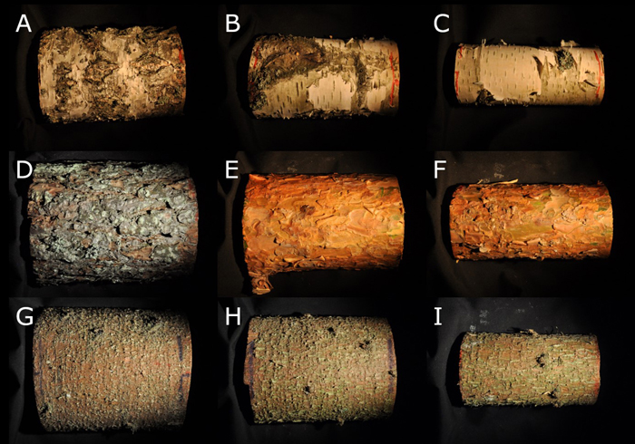
Fig. 1. Examples of silver birch (Betula pendula) (A–C), Scots pine (Pinus sylvestris) (D–F), and Norway spruce (Picea abies) (G–I ) stem bark samples from 1 m, 5 m, and 10 m heights, respectively.
2.2 Sample collection and storage
The stems were first marked at 1 m height with the main compass coordinates. Markings were made to keep track of the correct sides of the tree after the tree was cut down. After felling the tree, the tree was trimmed of branches. All study trees had a minimum height of 15 m. This ensured a minimum sample diameter of 5 cm at 10 m height of the tree. The minimum diameter or width of 5 cm in each sample was set to ensure that enough pixels of the sample were available for the data processing chain (see Section 2.4).
The collected samples were stored outside in cool March-April temperatures (approximately between 2–10 °C), covered and protected from weather conditions that could possibly alter the spectral properties of the samples. Measurements were carried out within 12 days from felling the trees.
2.3 Spectral measurements
We measured bi-directional reflectance factors (BRF) for the stem samples using a novel custom-built multiangular measurement set-up that utilized the Specim IQ mobile hyperspectral camera (Specim Ltd.) and a halogen light source. We constructed a multiangular system that operates along the principal plane with a fixed artificial source of illumination and is able to rotate 180° around the target (–90° and +90° of nadir) (Fig. 2). The system was restricted to the principal plane only, because the BRF typically varies the most along the principal plane. The rotation of the measurement arm was obtained through mechanically rotating it over the base. The view angle (i.e. angular position of the arm lever) was confirmed using a digital angle meter attached to the arm.
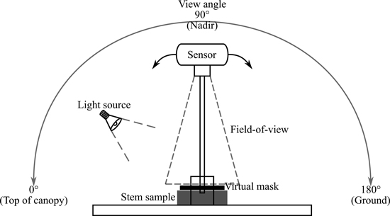
Fig. 2. Measurement set-up for the Specim IQ camera. View angle for the sensor could be set between 0–180° along the principal plane. The 0° would be top of canopy, 90° or nadir view angle was perpendicular to sample surface, and 180° was on the ground side of the sample. Small black rectangle represents the surface area of the sample used to calculate reflectance values (delineated by applying a virtual mask in the data processing). Grey rectangle represents the stem bark sample on the measurement table under the field-of-view of the sensor. One fixed light source at 40° angle (quartz tungsten halogen lamp) was used.
The Specim IQ mobile hyperspectral camera operates in the spectral wavelength range of 400–1000 nm, which covers the visible to near-infrared regions of the spectrum. The spectral resolution of the hyperspectral camera is 7 nm and it collects data for a total of 204 bands. The image size of the camera is 512 × 512 pixels with a field-of-view (FOV) of 31° × 31°. The entire hyperspectral image produced by the camera is therefore 512 × 512 pixels in 204 bands. The Specim IQ is based on a line scanner that performs the hyperspectral measurements with the pushbroom imaging principle. Behmann et al. (2018) have presented a more thorough technical description of the camera.
Two types of image data were collected. First, hyperspectral images were taken of each stem sample from six different view angles with one fixed illumination angle. A white reference was measured from the corresponding six view angles every 90 minutes. Maximum six samples could be measured within the 90-minute period. The white reference used in this study was a calibrated Spectralon® panel (25.4 × 25.4 cm) produced by Labsphere Inc., with a nominal reflectance of 99%. Second, high-resolution conventional red-green-blue (RGB) images were taken of each stem sample from the same view-illumination geometry as the hyperspectral images. The RGB images were taken with a Nikon D5000 camera and were used only for visualization purposes (i.e., to obtain a high resolution photo archive of measured samples collected through destructive means).
An overview of the measurement setup and view and illumination angles is provided in Fig. 2. In contrast to typical goniometer measurements (where zenith angles vary from –90° to +90°), we used a different angle notation convention to be consistent with typical satellite measurement geometry. In consequence of the zero-degree being vertically above the canopy in typical satellite measurement geometry, we consider the zero-degree to be along the table, towards the “top”-side of the sample (Fig. 2). Measurements made from 90° view angle will be referred to as nadir measurements (perpendicular to the sample surface).
The nominal illumination angle chosen for the measurements was 40°, which mimics what the solar zenith angle would be during the summer at midday in southern Finland. In addition, there is a previous study of woody tree structures that had similar conditions (even though measured outdoors) (Lang et al. 2002). Note that due to the conical geometry of the measurements (Fig. 2), the actual illumination angle was 40° ± 11° within the sample.
The artificial illumination we used was a 12 V 50 W quartz tungsten halogen (QTH) lamp with an aluminum reflector and a beam restrictor. A linear laboratory power supply (Twintex TP3020) was used to maintain a stable light output. Based on measurements with a Spectralon panel and a radiometrically calibrated spectrometer (ASD FieldSpec4), the total broadband irradiance of the lamp at the sample surface was 212 W m–2. The nominal 40° zenith angle for the lamp was achieved when the sample surface height was at 9 cm, and it is the same height at which the axis of rotation of the system was set at. If the sample or white reference panel was less than 9 cm in height, it was raised until the correct height was acquired. The measurement distance was set to 50 cm. The measurement distance allowed the 10-inch Spectralon® white reference target to fit the entire FOV of the Specim IQ camera. Sample placement was supported with a laser pointer to ensure approximate similarity between central alignment of samples.
Six nominal view angles were chosen: 29°, 58°, 65°, 90°, 115°, and 140° relative to the table. The idea was to obtain measurements at equal intervals between illumination direction (40°) and the direction opposite to light source (140°), to capture both hotspot and specular reflection behavior of the samples. Due to lamp geometry, the exact hotspot was not possible to achieve, and it was therefore replaced with two closest possible angles near the hotspot (29° and 58°). Similarly to the illumination angle, also the actual view angles of individual pixels within a sample varied ±10° from the nominal view angle.
In summary, 720 hyperspectral images and 720 high resolution RGB images were collected for 120 stem samples, together with necessary hyperspectral images of a white reference target for BRF calculations. Stray light effects were minimized by conducting all measurements in a windowless laboratory that had been painted in black with external light sources turned off. In addition, the multiangular measurement set-up had been spray painted with Nextel Velvet coating 811-21, which absorbs >97% of the light, independent of wavelength or the angle of incidence (Kwor et al. 2001). The table below the sample was not painted but was covered with black acrylic canvas that had directional hemispherical reflectance of 2% throughout the spectrum.
2.4 Data processing and analyses
To calculate BRF values for each pixel in the sample image, a data processing chain using Python programming language was developed for the raw data produced by the sensor (Specim IQ). The data processing chain allows the calculation and extraction of accurate pixel-specific reflectance information that is invariant to uneven spatial distribution of incident irradiance from the lamp.
The raw data of an image acquired with the Specim IQ consists of measured digital numbers (DN) for each pixel and the dark current data associated for each raw image. The dark current data is noise produced by the electronics within the sensor and needs to be removed from the captured DN values. In addition to taking the BRF of the measured white reference target to consideration in the computations, it is common that the integration times used by the sensor are different between the sample and the white reference. The following equation (referred to as the “pixel-by-pixel algorithm”) was used to calculate the BRF at a pixel level:

where:
DNsample is the digital number in the sample image,
DCsample is the dark current value for the sample image,
DNwhite_reference is the digital number of the white reference image,
DCwhite_reference is the dark current value for the white reference image,
BRFwhite_reference is the BRF for the white reference target obtainable from the calibration file provided by the manufacturer,
tsample is the integration time used to capture the sample, and
twhite_reference is the integration time used capture the white reference.
The data processing chain included creating virtual masks that select pixels, which represent purely the viewed area of the bark in each sample (i.e. no pixels from background or other non-bark regions). Each of the six measured angles were paired with their own virtual rectangular mask. The rectangular masks varied slightly in size (from approximately 8500 to 19 500 pixels) due to the viewed area changing with view angle. The masks for each view angle were made to fit the smallest stem sample out of the 120 for automating the process. Average mask size for a sample was approximately 3 × 15 cm. The pixels inside the masks were then used to calculate the BRF values with the pixel-by-pixel algorithm (Eq. 1).
Before the analyses, the data from wavelengths below 415 nm and above 925 nm were discarded. Instability in measured digital numbers was observed in those regions, when comparing the white reference images between measurements. The reason for the instability could be due to the material measured, source of illumination, short integration times, or limitations of the sensor technology within the camera itself. A previous evaluation study on Specim IQ (Behmann et al. 2018) reported similar limitations for the camera between 400–415 nm for some materials, and limitations for bands between 925–1000 nm were observable when measuring in direct sunlight (which could be comparable to the conditions present in this study).
In reporting our results, we will refer to the visible (VIS, 400–700 nm), and near-infrared (NIR, 700–1000) spectral regions.
2.5 Supervised machine learning classification
The algorithm used in this study was an implementation of a regularized linear SVM with stochastic gradient descent (SGD) learning. The reasoning behind selecting an estimator that utilizes a linear SVM with SGD learning is two-fold: one, it is scalable for very large machine learning problems, and two, it is computationally efficient for large amounts of samples. Similarly to other supervised classification algorithms, this linear SVM with SGD learning requires several hyperparameters (e.g. regularization term and maximum number of iterations). The hyperparameters were determined ad hoc and exhaustive grid search was used for tuning the hyperparameters. Furthermore, as SVMs are binary classifiers by nature, in order to achieve a multi-class classifier, the SVM utilizes a one-versus-all (OVA) method. The OVA method or scheme is such that for each of the three classes (birch, pine and spruce), a binary classifier is learned which discriminates between that and the other two classes. Finally, due to SGD being sensitive to feature scaling, the data were standardized (common requirement for many machine learning estimators) by removing the mean and scaling it to unit variance. A detailed study by Burges (1998) presents the mathematical formulations of the SVM algorithm. The linear SVM with SGD learning was constructed with Python programming language and a widely used machine learning library called scikit-learn (Pedregosa et al. 2011).
Training and test sets were created out of the pixel-level sample populations with a typical 80% and 20% ratio, respectively. Each class (birch, pine and spruce) had a balanced amount of observations (i.e. samples of spectra), and a random shuffle of the ordered samples was performed before splitting the data into training and test sets. The test set was set aside for the duration of training to assess performance later. In addition, the estimator was set to shuffle the training data after each pass (epoch) over the data during training. Instead of using a separate validation set for model evaluation, a k-fold cross-validation scheme was used to evaluate the performance of the model during training. A 5-fold cross-validation was used throughout the study. During the model optimization, the cross-validation score was used as an estimator to select the optimal model parameters for the separate test set. Finally, the test set (independent of the training dataset) was used together with the optimized model to predict class labels of unseen data, and to evaluate on the accuracy of the classification model. Accuracy of the predictions (i.e. success rate of classifying the correct tree species) were assessed through overall accuracy and class-specific accuracies. Overall accuracy is the ratio between the correct predictions by the model and the total number of observations.
Three different models (i.e. subsets of samples) were used in this study to run the classification and assess the classification accuracy of the algorithm: 1) pixel-wise classification based on nadir measurements, 2) pixel-wise classification based on all measurements, i.e., all view angles, and 3) sample-wise classification, i.e., using averaged spectra for each sample. In reporting our results, we will refer to the first subset (nadir model), second subset (all model), and third subset (mean model).
3 Results
3.1 Intra- and interspecific variation in nadir bark spectra
The results of the nadir measurements show that the two coniferous species, pine and spruce, had very similar spectra in VIS, especially between the wavelengths 415–550 nm (Fig. 3). In comparison to pine and spruce, the spectra of birch were in general distinctly higher (Fig. 3). Birch also displayed the highest standard deviation among the three species (Fig. 3). The mean BRF for birch varied between 0.22–0.55, for pine between 0.07–0.61, and for spruce between 0.07–0.53.
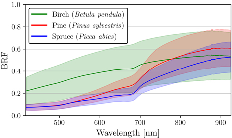
Fig. 3. Mean and standard deviation of reflectance (bi-directional reflectance factor, BRF) for silver birch (Betula pendula), Scots pine (Pinus sylvestris), and Norway spruce (Picea abies). Standard deviation was calculated between the pixel-level spectra derived from nadir measurements for each species.
Birch spectra were soil-like and increased monotonously as function of wavelength (Fig. 3). In addition, birch did not display typical vegetation characteristics strongly (e.g. strong absorption at red and blue wavelengths, or sharp rise at red edge). On the other hand, pine and spruce displayed some magnitude of red-edge effect that is typical for green vegetation (Fig. 3). The two conifer species displayed similar shapes of spectral signatures: The spectral signatures of spruce and pine were visually still distinguishable from one another even though there was clear overlap within VIS wavelengths (Fig. 3). Finally, the largest interspecific variation between the three species could be seen from the red-edge region to NIR (Fig. 3).
We analyzed if, and how, reflectance spectra of bark changes when moving upwards a tree trunk. The results for nine different spectral bands 492.4 nm, 559.8 nm, 664.6 nm, 704.1 nm, 740.5 nm, 782.8 nm, 834.8 nm, 864.7 nm, and 923.5 nm were used to illustrate the differences (Fig. 4A–I). In general, spruce displayed only small variation in spectra across the measured heights in all nine spectral bands (Fig. 4A–I). Birch displayed a similar trend for all nine bands: the BRF increased slightly when moving up along the stem (Fig. 4A–I). Perhaps the most significant result was discovered with pine, which had a clear increase in red and NIR BRFs when moving up along the stem of the tree (Fig. 4C–I). More specifically, pine showed a clear increase in reflectance between the heights of 1–5 m, after which BRF stabilized and remained similar between the heights of 5–10 m (Fig. 4C–I).
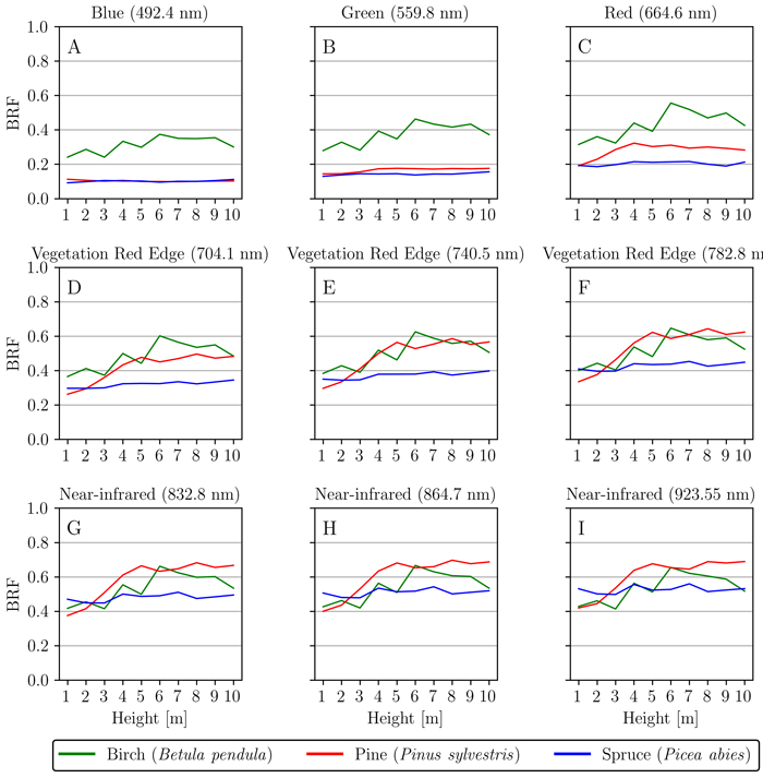
Fig. 4. Spatial variation of reflectance (bi-directional reflectance factor, BRF) along the tree height (1–10 m) for silver birch (Betula pendula), Scots pine (Pinus sylvestris), and Norway spruce (Picea abies). Nine wavelengths 492.4 nm (A), 559.8 nm (B), 664.6 nm (C), 704.1 nm (D), 740.5 nm (E), 782.8 nm (F), 834.8 nm (G), 864.7 nm (H) and 923.5 nm (I) were used to illustrate and analyze the changes in visible and near-infrared regions.
Finally, we looked at the reflectance differences between northern and southern sides of the trees. The sign and magnitude of the differences varied seemingly randomly between measurement heights, but when measurements of south and north sides were averaged over all heights and samples per species, some tendencies were found (Fig. 5). Pine and spruce had negligible differences between north and south in VIS, however, in the NIR region these species had on average 0.02 and 0.03 increased reflectance for the northern side, respectively (Fig. 5). Birch stood out in our results, as the south side samples had on average 0.10 increased reflectance for the entire VIS–NIR spectral region (Fig. 5). More specifically, south side samples of birch had on average 0.12 increased reflectance in VIS, and on average 0.07 increased reflectance in NIR (Fig. 5).
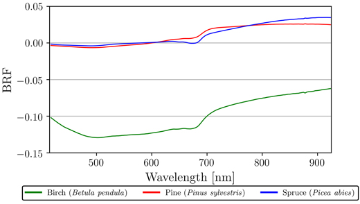
Fig. 5. Mean absolute differences in reflectance (bi-directional reflectance factor, BRF) between northern and southern sides of the measured trees for silver birch (Betula pendula), Scots pine (Pinus sylvestris), and Norway spruce (Picea abies). Measurements of north and south sides were averaged over all heights and samples per species. Order of difference: north minus south.
3.2 Intra and interspecific variation in multiangular bark spectra
In addition to the nadir measurements, we investigated the reflectance anisotropy of the three species along the principal plane for all six measured view angles (29°, 58°, 65°, 90°, 115°, and 140°). The results show that there were distinct differences in angular patterns of reflectance between the species. In contrast to the earlier results in Section 3.1, birch and pine behaved similarly to one another (Fig. 6A–B), while spruce had significantly different reflectance properties (Fig. 6C).
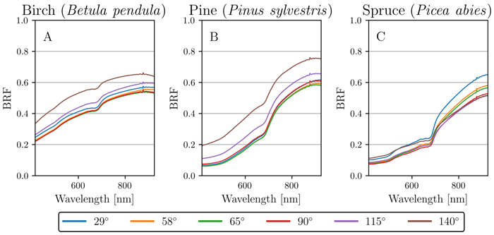
Fig. 6. Angular variation of reflectance (bi-directional reflectance factor, BRF) for silver birch (Betula pendula), Scots pine (Pinus sylvestris), and Norway spruce (Picea abies). Each plot (A, B, C) shows the mean reflectance for each measured angle (29°, 58°, 65°, 90°, 115° and 140°) per species: A) birch, B) pine, and C) spruce.
More specifically, birch and pine had noticeably increased reflectance in the forward-scattering directions (115° and 140° view angle) when compared to backward-scattering directions (Table 2). In contrast, spruce showed increased reflectance in the backward-scattering direction of 29° view angle, revealing a hotspot effect (Table 2). In addition to this hotspot effect, spruce displayed increased values in the forward-scattering direction of 140° view angle (i.e. having both hotspot and specular effects present) (Table 2). Closer inspection reveals that the 140° view angle for spruce had higher BRF in VIS, but the same BRF in NIR when compared to the nadir view (Table 2).
| Table 2. Relative mean percentage change of multiangular reflectance measurements for silver birch (Betula pendula), Scots pine (Pinus sylvestris), and Norway spruce (Picea abies). View angles are compared against the nadir (90°) measurements. Results are shown for three different wavelength regions: all wavelengths (415–925 nm), visible (415–925 nm), and near-infrared (415–925 nm). | |||||||||
| View angle (°) | All (415–925 nm) | Visible (415–700 nm) | Near-infrared (700–925 nm) | ||||||
| Birch | Pine | Spruce | Birch | Pine | Spruce | Birch | Pine | Spruce | |
| 29 | 6% | –4% | 32% | 7% | –6% | 35% | 5% | –0% | 26% |
| 58 | 1% | –9% | 10% | 1% | –12% | 10% | 2% | –3% | 11% |
| 65 | –1% | –10% | 6% | –1% | –13% | 6% | –1% | –4% | 7% |
| 90 | 0% | 0% | 0% | 0% | 0% | 0% | 0% | 0% | 0% |
| 115 | 12% | 26% | 6% | 14% | 35% | 10% | 10% | 10% | –2% |
| 140 | 34% | 82% | 22% | 40% | 113% | 34% | 23% | 30% | 0% |
3.3 Classification results
3.3.1 Based on nadir measurements
The overall accuracy for the pixel-level sample population based on the nadir measurements was 89.6% (Table 3). The best separation between the three species was acquired for birch (96.7%), which supports the results reported in Section 3.1 (i.e. birch having distinctly differing spectral signature in comparison to the two conifer tree species) (Table 3). Spruce and pine had accuracies of 92.1% and 80.1%, respectively (Table 3). Hence, the largest misclassification between species occurred for spruce and pine. Table 3 reports the overall accuracy and total number of samples used in more detail.
| Table 3. Classification results for three subset scenarios using a trained support vector machine classifier on a test set. The number of spectra in both training and test sets are given for each classification model. | ||||||
| Model | Number of spectra | Classification accuracy | Overall accuracy | |||
| Training set | Test set | Birch | Pine | Spruce | ||
| Nadir | 1 886 976 | 471 477 | 96.7% | 80.1% | 92.1% | 89.6% |
| All | 9 171 456 | 2 292 864 | 96.7% | 78.6% | 91.0% | 88.8% |
| Mean | 576 | 144 | 100.0% | 92.9% | 98.1% | 97.2% |
3.3.2 Based on all measurements
The results obtained using all six view angles were very similar to the smaller subset that only included pixels from nadir measurements (Section 3.3.1). The overall accuracy was 88.8%. Furthermore, the results showed that the classification of birch and spruce were at an acceptable accuracy for pixel-specific samples (96.7% and 91.0%, respectively), however pine had the lowest success rate (78.6%) (Table 3).
3.3.3 Based on mean spectra
We conducted a final estimation of tree species classification using SVMs on a dataset that averaged the spectra of all pixels in each sample into one spectrum. With this, we were able to decrease the number of samples down to 720 individual mean spectra (one per measured angle per stem sample), and perhaps more significantly, decrease the standard deviation and spectral variation within species. In this classification, the overall accuracy came to be 97.2% (Table 3).
4 Discussion
4.1 Intra- and interspecific variations in bark spectra from nadir measurements
The intraspecific variation in bark spectra was high when compared to, for example, leaves and needles of the same tree species published by Lukeš et al. (2013). Spruce displayed the lowest standard deviation (VIS–NIR) that could be explained by the most similar composition and texture between all species-specific samples (Fig. 1G–I). Pine had a slightly higher standard deviation than spruce in NIR region, which was most likely due to the clear visible changes in stem bark composition when inspecting lower and upper half of the tree trunk (Fig. 1D–F). Finally, birch showed the largest standard deviation (VIS–NIR) with distinct soil-like mean spectra that increased monotonously as a function of wavelength. The large intraspecific variation for birch could be explained by the substantial variations in structure and color between and within birch samples throughout the height of the stem (Fig. 1A–C). Birch samples presented a range of contrasting white to black colors (a typical characteristic for birch) with different stem surface textures. To summarize intraspecific variation, the within species reflectance variability was the lowest in VIS and the highest in NIR. A similar conclusion was reported by Asner (1998) but for different tree species.
We compared spectra with in situ data published by Lang et al. (2002), and the general shapes of mean spectra for the same tree species were found to be similar. Both this study and the results obtained from data published by Lang et al. (2002) showed distinct soil-like spectra for birch, distinguishable spectral signatures between the two conifer species, and noticeable red edge behavior for pine and spruce. The general shapes of mean spectra were similar, but the overall magnitudes differed, especially when comparing birch and spruce with the data published by Lang et al. (2002). The mean pine spectrum was nearly identical between the two datasets, and the mean birch and spruce spectra did fall within the standard deviation obtained in this study. Noteworthy is that the data by Lang et al. (2002) is the only openly available public repository for comparing silver birch, Scots pine, and Norway spruce. Furthermore, the within-species standard deviations were of similar magnitude to results reported in previous studies by Campbell et al. (2005), Hall et al. (2012), and Asner (1998), i.e., woody stem bark spectra of also other tree species were generally highly variable.
Interspecific variation in tree bark spectra was the largest in the red, red-edge and NIR spectral bands. Most overlap in spectra between-species was seen in VIS prior to the red wavelengths. Especially pine and spruce had overlap in this region. The largest spectral difference between pine and spruce could be found with samples collected from 5–10 m stem height, between red to NIR spectral bands (Fig. 4C–I). Birch had the greatest between-species difference to the two coniferous species in the visible spectral bands of red, green and blue (Fig. 4A–C). More specifically, spruce showed no trends along the height of the tree for all analyzed spectral bands (Fig. 4A–I), and this is possibly supported by spruce stem bark not changing significantly (e.g. color or texture) along different heights of the stem for both sampled trees (Fig. 1G–I). On the other hand, both pine trees had a clear gradual change (texture, structure and color) along the stem, which affected the BRF at red–NIR spectral wavelengths (Fig. 4C–I). The visible changes along the different heights of the stem were typical for pine (e.g. color changing from brownish-gray (Fig. 1D) to more orange-red tones (Fig. 1F)). Finally, birch showed a minor increasing trend in reflectance for all examined spectral bands when moving up the tree stems (Fig. 4A–I). This small increase could be the result of the sampled trees having darker and coarser stem bark texture closer to the ground (Fig. 1A), while finding relatively larger surface areas of smooth texture and typical whitish color when going towards the top of canopy (Fig. 1C). Finally for the interspecific variation, the modest red-edge effect (absorption at blue and red wavelengths, and a rise near the red edge) that was displayed by spruce and pine could be supported by the external visible green vegetation (mosses and lichens) that grew occasionally on top of the bark. Pine also had a clear gradient in its bark features: on the lower parts of the trunk there were slightly more external lichen or mosses growing than higher up on the trunk and, higher up along the stem, greenish characteristics under the topmost bark layer became more common.
When we compared the differences in averaged reflectance of northern and southern sides of the measured trees, pine and spruce had very similar results, i.e., the north side samples had slightly stronger reflectance in NIR. This tendency could be the result of the two cardinal sides having different environmental conditions (e.g., illumination and moisture) for external vegetation growth (mosses and lichens) or bark structural development. On the other hand, birch displaying a very large difference in favor of the southern side, is explained by one of the two sampled birches (birch 2) having noticeably whiter south side of the stem. This was evident after visually inspecting images of measured samples from the two birch trees. The birch with the most reflective south side (birch 2) grew at the very edge of the forest stand with no shade from the surrounding trees on the southeastern side. Thus, the environmental conditions could be a potential explanation for the observed large difference for this particular tree.
4.2 Variations in multiangular bark spectra
Prior to this study there are no publications of multiangular spectral properties of stem bark, and our results are novel. Increased reflectance in forward-scattering directions, i.e., specular reflection, for pine and birch was likely caused by the smooth surface textures on their stem bark. Noteworthy is that, based on visual judgement, both birch and pine had smoother surface areas on the stem bark when moving higher up on the stem (e.g., Fig. 1C and Fig. 1F). The specular reflection could also be observed in practice already during the measurements, because the integration times used for acquiring images in the forward-scattering angles had to be made much shorter to avoid over-exposure. In contrast to pine and birch that behaved similarly to one another, spruce displayed clearly different angular variations in spectra due to the structural and textural characteristics of its stem bark. Spruce stem bark was noticeably coarser and had rough surface properties. The surface structure of spruce stem bark could be described as having small fragile outward-bending structures that were aligned so that when imaged from forward-scattering angles, the structures created subtle shadows throughout the sample. The shadows however constituted to a significant enough portion of the surface area seen by the sensor, which possibly explains the lower overall reflectance in the forward-scattering angles (when compared to the hotspot effect in the backward-scattering side). The two highest angular effects for spruce were found at 29° and 140°, which again suggest that spruce had a more complex angular behavior at surface structural level when compared to pine and birch.
4.3 Potential and limitations of bark spectra for classification
The overall accuracy for classifying tree species was strong for pixel-wise models derived from nadir and all hyperspectral images, taking into consideration that there was high spectral variability within-species and overlap in spectra between-species. The classifier was able to fit the linear SVM (i.e. solve the inseparability problem) in such a way, that it could classify the three tree species effectively. Hence, soft-margin linear separation was possible, even though the pixel samples represent varying surface conditions (due to the very high spatial resolution acquired for each pixel) with overlapping spectra between-species.
Perhaps the most significant result obtained from the nadir and all pixel models was that it showed the scalability of a linear SVM with SGD learning for complete VIS–NIR spectral observations. In other words, the models were able to classify pixel-specific spectra with an acceptable accuracy for future applications that might need solutions for large data. As the pixel-specific accuracy also revealed the limitation in separating pine and spruce, the final model that utilized mean spectra per sample resulted in very high and reliable classification accuracy. The separation of pine and spruce could be potentially further enhanced in the future by using images from stem heights where the spectra between-species differ as much as possible (i.e. not comparing lower parts of the trunk where the reflectance properties are nearly identical between, for example, spruce and pine).
The classification results are rather promising and show positive indications that hyperspectral images can be used, for example, in applications related to autonomous forestry machinery (Billingsley et al. 2008; Bergerman et al. 2016), forest inventories that utilize mobile imaging (Molinier et al. 2016), or mobile phone-based applications for identifying plant species in the field (Pl@ntNet 2020). It seems that the spectra obtained from hyperspectral images contain valuable species-specific information that machine learning algorithms like the SVM can use optimally even at pixel level. In fact, spatial averaging of obtained spectra improved classification results even further. Notably, this study shows that it is possible to identify common boreal tree species based on their stem bark spectra using images from mobile hyperspectral cameras.
4.4 Stem bark spectra in future research
The influence of woody tree structures on canopy reflectance can differ widely from one forest biome to another. Noteworthy is that total canopy reflectance is possibly more affected by woody tree structures in boreal forests than, for example, temperate forests. Boreal forests have large between-crown gaps (Nilson 1999), whilst temperate forests canopies can be dense and gap fractions in them dominated by small within-crown gaps (Chianucci 2020). Even in boreal forests, it is difficult to detect woody tree structures, such as stems and branches, directly from coarse spatial resolution optical remote sensing images (when measured above canopy). With higher spatial resolution and in oblique viewing angles, a larger contribution is more likely caused by branches. Hence, research on spectral properties of branches could be very useful in combination with knowledge on the spectral characteristics of stem bark. In addition, in situ mapping of tree species with mobile sensors (such as the one used in this study) would benefit from spectral libraries of stem bark. Finally, information on stem bark is also needed in radiative transfer modeling of forests, and it can potentially be utilized also in close-range sensing methods, e.g., state-of-the-art autonomous forest inventory drones operating under the forest canopy.
Future measurements could be directed at progressing from a controlled laboratory setting to conduct similar measurements in the field in more natural conditions. Wider sampling of living trees could aid in drawing more accurate generalizations across larger areas. Method development could be aided with state-of-the-art deep learning methods where both the spectra and the texture of the stem bark are considered for even more accurate classification results.
Acknowledgements
We thank Ms. Sanna Ervasti, the city forester of Vantaa, for collaboration in acquisition of the sample trees. This study was funded by the Academy of Finland (grants 286390 and 323004). This study also received funding from the European Research Council (ERC) under the European Union’s Horizon 2020 research and innovation programme (grant agreement No 771049). The text reflects only the authors’ view and the Agency is not responsible for any use that may be made of the information it contains.
References
Asner G.P. (1998). Biophysical and biochemical sources of variability in canopy reflectance. Remote Sensing of Environment 64(3): 234–253. https://doi.org/10.1016/S0034-4257(98)00014-5.
Behmann J., Acebron K., Emin D., Bennertz S., Matsubara S., Thomas S., Bohnenkamp D., Kuska M.T., Jussila J., Salo H., Mahlein A.-K., Rascher U. (2018). Specim IQ: evaluation of a new, miniaturized handheld hyperspectral camera and its application for plant phenotyping and disease detection. Sensors 18(2) article 441. https://doi.org/10.3390/s18020441.
Bergerman M., Billingsley J., Reid J., van Henten E. (2016). Robotics in agriculture and forestry. In: Siciliano B., Khatib O. (eds.). Springer handbook of robotics. Springer Handbooks, Springer, Cham. p. 1463–1492. https://doi.org/10.1007/978-3-319-32552-1_56.
Billingsley J., Visala A., Dunn M. (2008). Robotics in agriculture and forestry. In: Siciliano B., Khatib O. (eds.). Springer handbook of robotics. Springer, Berlin, Heidelberg. p. 1065–1077. https://doi.org/10.1007/978-3-540-30301-5_47.
Burges C.J.C. (1998). A tutorial on support vector machines for pattern recognition. Data Mining and Knowledge Discovery 2(2): 121–167. https://doi.org/10.1023/A:1009715923555.
Campbell S.A., Borden J.H. (2005). Bark reflectance spectra of conifers and angiosperms: implications for host discrimination by coniferophagous bark and timber beetles. The Canadian Entomologist 137(6): 719–722. https://doi.org/10.4039/N04-082.
Chianucci F. (2020). An overview of in situ digital canopy photography in forestry. Canadian Journal of Forest Research 50(3): 227–242. https://doi.org/10.1139/cjfr-2019-0055.
Dangel S., Kneubuhler M., Kohler R., Schaepman M., Schopfer J., Schaepman-Strub G., Itten K. (2003). Combined field and laboratory goniometer system – FIGOS and LAGOS. In: International Geoscience and Remote Sensing Symposium (IGARSS) Vol. 7. p. 4428–4430. https://doi.org/10.1109/IGARSS.2003.1295536.
Gewali U.B., Monteiro S.T., Saber E. (2018). Machine learning based hyperspectral image analysis: a survey. arXiv. https://arxiv.org/abs/1802.08701. [Cited 19 Feb 2020].
Gualtieri J.A., Cromp R.F. (1999). Support vector machines for hyperspectral remote sensing classification. In: 27th AIPR Workshop: Advances in Computer-Assisted Recognition. SPIE. p. 221–232. https://doi.org/10.1117/12.339824.
Hadlich H.L., Durgante F.M., dos Santos J., Higuchi N., Chambers J.Q., Vincentini A. (2018). Recognizing Amazonian tree species in the field using bark tissues spectra. Forest Ecology and Management 427: 296–304. https://doi.org/10.1016/j.foreco.2018.06.002.
Hall F.G., Huemmrich K.F., Strebel D.E., Goetz S.J., Nickeson J.E., Woods K.D. (1992). Biophysical, morphological, canopy optical property, and productivity data from the superior national forest. NASA Technical Memorandum 104568. NASA Goddard Space Flight Center, Greenbelt, MD, USA. 150 p.
Halme E., Pellikka P., Mõttus M. (2019). Utility of hyperspectral compared to multispectral remote sensing data in estimating forest biomass and structure variables in Finnish boreal forest. International Journal of Applied Earth Observation and Geoinformation 83 article 101942. https://doi.org/10.1016/j.jag.2019.101942.
Hovi A., Raitio P., Rautiainen M. (2017). A spectral analysis of 25 boreal tree species. Silva Fennica 51(4) article 7753. https://doi.org/10.14214/sf.7753.
Juola J. (2019). Multi-angular measurement of woody tree structures with mobile hyperspectral camera. Master’s Thesis, Aalto University, School of Engineering, Department of Built Environment, Espoo, Finland. http://urn.fi/URN:NBN:fi:aalto-201908254904. [Cited 10 Jan 2020].
Kuusk A., Kuusk J., Lang M. (2009). A dataset for the validation of reflectance models. Remote Sensing of Environment 113(5): 889–892. https://doi.org/10.1016/j.rse.2009.01.005.
Kwor E.T., Matteï S. (2001). Emissivity measurements for Nextel Velvet Coating 811-21 between –36 °C and 82 °C. High Temperatures – High Pressures 33(5): 551–556. https://doi.org/10.1068/htwu385.
Lang M., Kuusk A., Nilson T., Lükk T., Pehk M., Alm G. (2002). Reflectance spectra of ground vegetation in sub-boreal forests. Tartu Observatory, Estonia. http://www.aai.ee/bgf/ger2600/. [Cited 7 Feb 2020].
Lukeš P., Stenberg P., Rautiainen M., Mõttus M., Vanhatalo K.M. (2013). Optical properties of leaves and needles for boreal tree species in Europe. Remote Sensing Letters 4(7): 667–676. https://doi.org/10.1080/2150704X.2013.782112.
Malenovský Z., Martin E., Homolová L., Gastellu-Etchegorry J.P., Zurita-Milla R., Schaepman M.E., Clevers J., Cudlín P. (2008). Influence of woody elements of a Norway spruce canopy on nadir reflectance simulated by the DART model at very high spatial resolution. Remote Sensing of Environment 112(1): 1–18. https://doi.org/10.1016/j.rse.2006.02.028.
Mantero P., Moser G., Serpico S.B. (2005). Partially supervised classification of remote sensing images through SVM-based probability density estimation. IEEE Transactions on Geoscience and Remote Sensing 43(3): 559–570. https://doi.org/10.1109/TGRS.2004.842022.
Melgani F., Bruzzone L. (2004). Classification of hyperspectral remote sensing images with support vector machines. IEEE Transactions on Geoscience and Remote Sensing 42(8): 1778–1790. https://doi.org/10.1109/TGRS.2004.831865.
Molinier M., López-Sánchez C.A., Toivanen T., Korpela I., Corral-Rivas J.J., Tergujeff R., Häme T. (2016). Relasphone – mobile and participative in situ forest biomass measurements supporting satellite image mapping. Remote Sensing 8(10) article 869. https://doi.org/10.3390/rs8100869.
Mountrakis G., Im J., Ogole C. (2011). Support vector machines in remote sensing: a review. ISPRS Journal of Photogrammetry and Remote Sensing 66(3): 247–259. https://doi.org/10.1016/j.isprsjprs.2010.11.001.
Nilson T. (1999). Inversion of gap frequency data in forest stands. Agricultural and Forest Meteorology 98–99: 437–448. https://doi.org/10.1016/S0168-1923(99)00114-8.
Pal M., Mather P.M. (2005). Support vector machines for classification in remote sensing. International Journal of Remote Sensing 26(5): 1007–1011. https://doi.org/10.1080/01431160512331314083.
Pedregosa F., Varoquaux G., Gramfort A., Michel V., Thirion B., Grisel O., Blondel M., Prettenhofer P., Weiss R., Dubourg V., Vanderplas J., Passos A., Cournapeau D., Brucher M., Perrot M., Duchesnay E. (2011). Scikit-learn: machine learning in python. JMLR 12: 2825–2830. http://www.jmlr.org/papers/volume12/pedregosa11a/pedregosa11a.pdf. [Cited 20 Jan 2020].
Pl@ntNet (2020). https://plantnet.org/en/. [Cited 24 Feb 2020].
Rautiainen M., Lukeš P., Homolová L., Hovi A., Pisek J., Mõttus M. (2018). Spectral properties of coniferous forests: A review of in situ and laboratory measurements. Remote Sensing 10(2) article 207. https://doi.org/10.3390/rs10020207.
Roosjen P.P.J., Clevers J.G.P.W., Bartholomeus H.M., Schaepman M.E., Schaepman-Strub G., Jalink H., van der Schoor R., de Jong A. (2012). A laboratory goniometer system for measuring reflectance and emittance anisotropy. Sensors (Switzerland) 12(12): 17358–17371. https://doi.org/10.3390/s121217358.
Shaharum N.S.N., Shafri H.Z.M., Ghani W.A.W.A., Samsatli S., Yusuf B., Al-Habshi M.M. A., Prince H.M. (2018). Image classification for mapping oil palm distribution via support vector machine using scikit-learn module. International Archives of the Photogrammetry, Remote Sensing and Spatial Information Sciences – ISPRS Archives 42: 139–145. https://doi.org/10.5194/isprs-archives-XLII-4-W9-133-2018.
Stenberg P., Lukeš P., Rautiainen M., Manninen T. (2013). A new approach for simulating forest albedo based on spectral invariants. Remote Sensing of Environment 137: 12–16. https://doi.org/10.1016/j.rse.2013.05.030.
Suomalainen J., Hakala T., Peltoniemi J., Puttonen E. (2009). Polarised multiangular reflectance measurements using the Finnish geodetic institute field goniospectrometer. Sensors 9(5): 3891–3907. https://doi.org/10.3390/s90503891.
Verrelst J., Schaepman M.E., Malenovský Z., Clevers J.G.P.W. (2010). Effects of woody elements on simulated canopy reflectance: Implications for forest chlorophyll content retrieval. Remote Sensing of Environment 114(3): 647–656. https://doi.org/10.1016/j.rse.2009.11.004.
Total of 34 references.
