Karol Bronisz  ,
Michał Zasada
,
Michał Zasada
Taper models for black locust in west Poland
Bronisz K., Zasada M. (2020). Taper models for black locust in west Poland. Silva Fennica vol. 54 no. 5 article id 10351. https://doi.org/10.14214/sf.10351
Highlights
- Seven taper models with different numbers of estimated parameters were analysed
- Section diameter and volume was modelled using fixed and mixed-effects modelling approaches
- The variable-form taper model with eight estimated parameters fitted the data the best
- The lowest error for volume prediction was achieved for the fixed-effects taper model.
Abstract
The diameter at any point on a stem and tree volume are some of the most important types of information used in forest management planning. One of the methods to predict the diameter at any point on a stem is to develop taper models. Black locust (Robinia pseudoacacia L.) occurs in almost all forests in Poland, with the largest concentration in the western part of the country. Using empirical data obtained from 13 black locust stands (48 felled trees), seven taper models with different numbers of estimated parameters were analysed for section diameters both over and under bark using fixed and mixed-effects modelling approaches. Assuming a lack of additional measurements, the best fitted taper models were used for the prediction of over bark volume using both methods. The predicted volume was compared with the results from different volume equations available for black locust. The variable-form taper model with eight estimated parameters fitted the data the best. The lowest root mean square error for volume prediction was achieved for the elaborated fixed-effects taper model (0.0476), followed by the mixed-effects taper model (0.0489). At the same time, the difference between the volume relative errors achieved based on the taper models does not differ significantly from the results obtained using the volume equations already available for black locust (two of the three analysed).
Keywords
taper;
Robinia pseudoacacia;
mixed-effects models;
section diameter over and under bark;
volume prediction
-
Bronisz,
Institute of Forest Sciences, Warsaw University of Life Sciences-SGGW, Nowoursynowska 159, PL 02-776 Warsaw, Poland
E-mail
karol.bronisz@wl.sggw.pl
-
Zasada,
Institute of Forest Sciences, Warsaw University of Life Sciences-SGGW, Nowoursynowska 159, PL 02-776 Warsaw, Poland
 https://orcid.org/0000-0002-4881-296X
E-mail
Michal.Zasada@wl.sggw.pl
https://orcid.org/0000-0002-4881-296X
E-mail
Michal.Zasada@wl.sggw.pl
Received 10 April 2020 Accepted 18 September 2020 Published 1 October 2020
Views 92656
Available at https://doi.org/10.14214/sf.10351 | Download PDF

1 Introduction
The southeastern part of the United States is a natural area for the growth for black locust (Robinia pseudoacacia L.). The centre of the range of this tree species is located at altitudes of 150 to 1500 metres above sea level in Appalachia (Fowells 1965). The species was introduced to Europe by Jean Robin (Nowiński 1977). In the initial phase of its introduction, black locust was mainly grown as a park tree. The potential distribution of black locust throughout European countries is mainly in the United Kingdom, Germany, France, the Netherlands, Belgium, Italy and Switzerland (Li et al. 2014). Moreover, black locust is the most widely planted species in Hungary, covering 23% of the country’s total forest area (Rédei et al. 2012). This species is also important in Turkey, where it has been planted over an area of 3000 ha since 1995 (Yüksek 2012), and it is considered to be a favourable tree species for soil reclamation and the regeneration of disturbed sites (Bolat et al. 2015).
Black locust was brought to Poland in 1806 (Tokarska-Guzik 2005). Currently, the species occurs in almost all forests in Poland, with the largest concentration in the western part of the country. Black locust stands occupy over 273 000 ha of Polish forests and provide 84 000 cubic metres of wood annually (Wojda et al. 2015). One of the reasons for the interest in this species is the demand for black locust wood: in areas with a high share of this species, wood demand outweighs the supply. In addition, black locust wood is exported from Poland to the Netherlands (Wojda et al. 2015). Black locust has also been successfully used for over 30 years in the reclamation of areas around coal mines and power plants (Wojda et al. 2015; Jagodziński et al. 2018; Horodecki et al. 2019). To date, the distribution of black locust throughout Europe appears to be mostly limited by low temperatures, but global warming might enhance its growth in colder areas (Nadal-Sala et al. 2019). In the context of climate change, black locust wood has been utilized in a new structural system known as the Triakonta Connection System, which is a modular wood-based, carbon sequestering system designed to reduce landfill waste (Womer 2012). However, when defining the role of this tree species in a given forest ecosystem, it should be remembered that it is an invasive tree species (Radtke et al. 2013; Vítková et al. 2017).
Information about the tree stem shape, as well as the volume (whole stem and its various assortments), is one of the most important factors used in forest management planning, forest operations and the timber industry. One of the possibilities for defining the shapes of trees is to develop taper models, which allow the diameter to be determined at any place on the stem. This information then enables the calculation of volume, biomass (Brooks et al. 2007) and the amounts of various wood products (Dudzińska 2003). One group of taper models are linear models that describe the shape of a tree using a certain number of diameters at different relative tree heights (Lappi 1986; Socha 2002; Socha and Kubik 2005). A linear model, which was developed based on 15 relative tree heights determined for 15 sections of equal lengths in the tree volume, was the first Polish taper model (Bruchwald 1980). Notwithstanding, nonlinear models represent the largest group of solutions found in the literature. In the simplest case, the shape of a stem can be mapped using a single mathematical function (Kozak 1988). This function may be polynomial (Munro 1966; Kozak et al. 1969), power (Demaerschalk 1972), trigonometric (Bi 2000; Socha 2002) or exponential (Biging 1984). It is also possible to use a variable shape equation (Riemer et al. 1995), assuming that the shape varies along the tree (Lee et al. 2003). Nonlinear taper models composed of two or more segments approximated with different geometric solids are also available (Max and Burkhart 1976).
The section diameters used to elaborate taper models are characterized by a hierarchical structure, which contains information about individual diameters, trees and plots. The mixed-effects modelling approach is a possible solution to handle such data (Pinheiro and Bates 2013). The fixed parts of these models allow the data for a typical basic group (e.g., tree or plot) to be modelled, whereas the random part describes the difference between each group and a typical value, thus providing descriptions of the specific relationships among all groups of the dataset (Mehtätalo and Lappi 2020). During taper modelling based on the mixed-effects modelling approach, various strategies can be adopted. One possibility is to define random effects on the individual tree level (without modelling the autocorrelation). This approach allows the largest possible proportion of the between-tree variation to be explained (Diéguez-Aranda et al. 2006; de-Miguel et al. 2012). Mixed-effects models also enables to include both: tree and plot grouping level (multilevel mixed-effect models) into random effects (Lappi 1986; Arias-Rodil et al. 2015). In addition, convergence problems should also be considered during taper model fitting (Yang et al. 2009). Other elements worth considering are the practical use of the created model (Arias-Rodil et al. 2015). In this case, where additional measurements of the section diameter are necessary for the prediction of random effects, the predictions can be averaged over the estimated distribution of the random effects. Another possibility is to apply fixed effects predictions of the mixed-effect model (de-Miguel et al. 2012). However, fixed effects predictions based on the mixed-effect model, assuming that random parameters are zero, can lead to larger errors and higher bias for section diameter prediction (Pukkala et al. 2019). Therefore, taking into account practical considerations and obtained errors, it is also worth considering the usage of a simple fixed-effects model for taper modelling (Arias-Rodil et al. 2015).
Considering the above issues, the objectives of this study were to (i) fit selected taper models to the section diameters over bark and under bark as fixed-effects models, (ii) for both section diameters, fit the best taper model as the mixed-effects model with tree and plot as grouping levels, (iii) compare both fitting strategies for the section diameters over bark and under bark, and (iv) compare both strategies for determining the tree volume over bark, considering the available volume equations for black locust (Sopp and Kolozs 2000; Moshki and Lamersdorf 2011; Lockow and Lockow 2015).
2 Material and methods
2.1 Study site and sample plots
The empirical data were collected from 13 black locust stands located in west Poland (Sulechów, Sława Śląska and Gubin forest districts, 52°08’–51°30´N, 15°23’–16°14´E, Fig. 1, Table 1). Sample plots were located on oligotrophic sites typical for black locust (i.e., fresh mixed coniferous forest and fresh mixed broadleaved forest, according to the Polish forest site classification). The research area was located in a transition zone from maritime to continental types within a temperate climate (Martyn 2000). The mean annual temperature reaches 10 °C. January is the coldest month with an average temperature slightly below –1 °C. The highest average temperature is recorded in July (20 °C). The average annual rainfall rarely exceeds 550 to 600 mm.
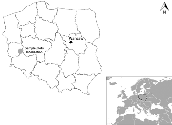
Fig. 1. Location of black locust sample plots in west Poland.
| Table 1. Summary characteristics of the black locust sample plots located in west Poland: average stand age (A, years), sample plot area (P, m2), stocking (N, trees ha–1), basal area at breast height (BA, m2 ha–1), average diameter at breast height (Dg, cm), and average height (Hg, m). | |||||
| Minimum | Maximum | Mean | Median | Stand. Dev. | |
| A | 16 | 85 | 50 | 50 | 21 |
| P | 864 | 5944 | 2359 | 1914 | 1278 |
| N | 167 | 1134 | 586 | 507 | 304 |
| BA | 10.06 | 40.52 | 21.73 | 20.53 | 7.72 |
| Dg | 11.47 | 43.94 | 23.94 | 25.23 | 9.08 |
| Hg | 9.84 | 27.19 | 20.3 | 21.18 | 5.19 |
The borders of the chosen rectangular sample plots were permanently marked in the field. The size of each plot was set in such a way that it comprised at least 100 trees. The diameter at breast height (DBH) of all live trees (accuracy 0.1 cm) was measured on all plots, as well as at 25 heights (H) from height sample trees (accuracy 0.01 m), to build a local height-diameter model.
2.2 Tree level data
At each sample plot, 3 to 6 sample trees representing the whole range of diameter structure were chosen and felled. In total, 48 sample trees were used for further analyses (Fig. 2). The height of the analysed trees varied from 7.5 m to 27.9 m, and the DBH varied from 8.1 cm to 46.7 cm; the mean values of these parameters were 19.99 m and 24.05 cm, respectively (Table 2).
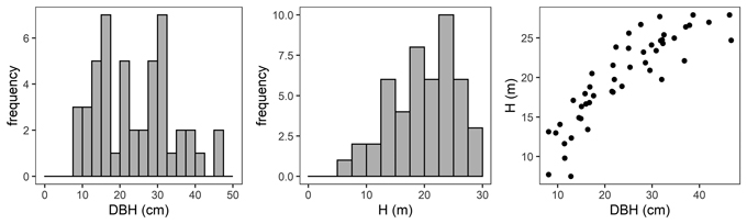
Fig. 2. Diameter at breast height (DBH) distribution (left), height distribution (H, middle) and H-DBH relationship (right) of black locust sample trees.
| Table 2. Characteristics of black locust sample trees. Diameter at breast height (DBH, cm), tree height (H, m), section diameter over bark (D, cm), section diameter under bark (d, cm) and reference tree volume over bark (VR, m3). | |||||
| Minimum | Maximum | Mean | Median | Stand. Dev. | |
| DBH | 8.1 | 46.7 | 24.05 | 22.98 | 10.29 |
| H | 7.5 | 27.9 | 19.99 | 20.7 | 5.54 |
| D | 0.3 | 54.8 | 16.19 | 15.35 | 10.13 |
| d | 0.15 | 49.25 | 13.93 | 13.30 | 8.57 |
| VR | 0.0212 | 1.8056 | 0.5421 | 0.3959 | 0.4681 |
Felled trees were measured section-wise (1 m section length – measurements at 0m, 1 m, 2 m, etc.) to obtain their section diameter over bark. Stem discs from the lower end of each section were taken to determine the section diameter under bark. As a result, 975 section diameters over bark and 792 section diameters under bark were obtained (Fig. 3). In addition, based on the section-wise measurements, reference volumes over bark for sample trees were calculated using the sectional Smalian’s equation (Eq. 11, Table 2).
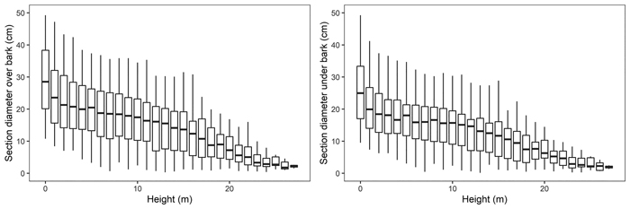
Fig. 3. Black locust sample trees section diameters over bark (left) and under bark (right).
2.3 Fixed-effects taper models
Considering the practical application of the elaborated taper models, we chose solutions that used DBH and H (as independent variables) to define the tree shape, which, as a consequence, translated into the possibility of determining its volume. The analysed taper models were fitted in relation to squared section diameters. This solution allows to reduce bias for the cross-sectional area and volume prediction (Bruce et al. 1968; de-Miguel et al. 2012). Seven candidate taper models, which have shown good performance in previous studies (Rojo et al. 2005; de-Miguel et al. 2012; Bronisz and Zasada 2019) and have different numbers of parameters (from 2 to 8), were taken into account:
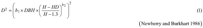
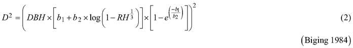
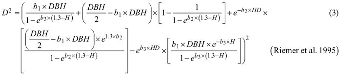
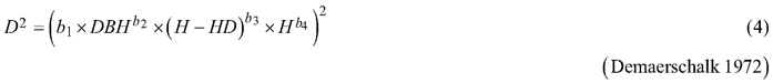
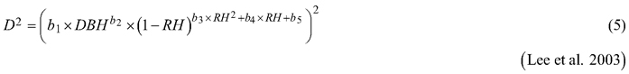
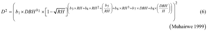
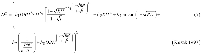
where D is section diameter over bark (cm), DBH is diameter at breast height over bark (cm), H is tree height (m), HD is section height (m), RH is relative height (HD/H), and t is relative breast height (1.3/H).
During the first step of the analyses the abovementioned taper models 1–7 were fitted using a nonlinear ordinary least squares approach using gnls function from nlme R package (Pinheiro et al. 2020). Analyses were carried out for both the over bark (D) and under bark (d) section diameters. Fitted taper models were compared based on goodness-of-fit measures such as:
• coefficient of determination (R2):

where ![]() is the measured section diameter,
is the measured section diameter, ![]() is the modelled section diameter, and
is the modelled section diameter, and ![]() is the mean value of the measured section diameter,
is the mean value of the measured section diameter,
• mean error (ME):

where n is the number of section diameters, and
• Akaike information criterion (AIC):

where ![]() is the logarithm of the likelihood function for the estimated parameter and p is the number of model parameters.
is the logarithm of the likelihood function for the estimated parameter and p is the number of model parameters.
2.4 Mixed-effects taper models
The best taper models for section diameter over bark and under bark (chosen from models 1–7) were fitted using a mixed-effects modelling approach. Given the value of the obtained Akaike information criterion (AIC) (Eq. 10), the possibility of defining different random parameters was assessed, with a maximum of three parameters on both: trees and plots as grouping levels. Such a definition of parameters allowed us to avoid highly correlated random effects and convergence problems, while also allowing us to consider both the between-tree and between-plot variation in the different parts of the stem (de-Miguel et al. 2012).
In addition, the obtained Pearson residuals alike for fixed-effects and mixed-effects taper models were analysed graphically based on their relationships with the section diameter and relative height. During analyses heteroscedasticity in the residuals was also included. In the case of heteroscedastic data, analysing likelihood ratio test and solutions containing various functions and predictors, a power-type variance function with tree diameter at breast height as a predictor were applied (De-Miquel et al. 2012; Arias-Rodil et al. 2015; Bronisz and Mehtätalo 2020).
2.5 Tree volume
The reference over bark volumes of sample trees were calculated based on the 1 m section-wise Smalian’s equation:

where RV is the reference volume (m3), ls is the length of the section (m), g0, gn, g1, g2, g3 and gn–1 are the basal areas at the beginning and end of individual sections (m2), and Va is the volume of the last section (m3).
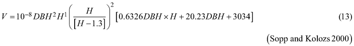
During volume calculation, the best fixed-effects (first strategy) and mixed-effects taper models (second strategy) were used. Given the practical application of the elaborated mixed-effects taper model (de-Miguel et al. 2012), it was assumed that additional measurements of section diameter, which are necessary for the prediction of random effects, were not available. Therefore, as a part of the second strategy, we predicted volume based on the fixed part of a mixed-effects model under the condition that the random effects were equal to zero. For both strategies, the predicted stem volume was computed by numerical integration (R-function integrate, Arias-Rodil et al. 2015; Mehtätalo and Lappi 2020). The accuracy of such a volume was compared to the reference tree volume (RV, Eq. 11), and the volume achieved based on different available equations for black locust:


The basis for the accuracy comparison were:
• a 95% confidence interval (R-function summarySE) for the relative error (RE):
![]()
where RV is the reference volume (m3) and V is the volume (m3) achieved based on elaborated taper models (both strategies) and different available equations for black locust (Eq. 12–14).
• root mean square error (RMSE):

where nv is the number of sample trees.
All analyses were performed using R 3.6.2 software (R Core Team 2020), RStudio 1.2.5033 (RStudio team 2015), with the ggplot2 (Wickham 2016) and nlme (Pinheiro et al. 2020) packages.
3 Results
3.1 Section diameter – fixed-effects taper model
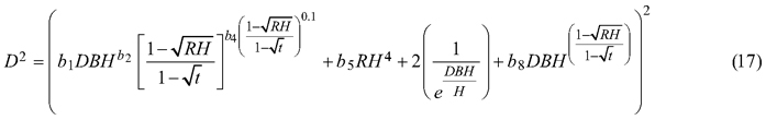
For both section diameters over and under bark, the lowest R2 and highest ME and AIC values (Table 3) were obtained during fitting the fixed-effects taper model that included three parameters (Eq. 3). The highest R2 and the lowest ME and AIC values were achieved for the taper model that included eight parameters (Eq. 7). For section diameters over bark those goodness-of-fit measures for the best fitted taper model (Eq. 7) equal 0.962, –1.528 and 11 312, respectively (Table 3).
| Table 3. Goodness-of-fit measures for the analysed fixed-effects taper models for black locust: R2 – coefficient of determination (Eq. 8), ME – mean error (Eq. 9), and AIC – Akaike information criterion (Eq. 10). Model nr. 1 – Newberry and Burkhart 1986, nr. 2 – Biging 1984, nr. 3 – Riemer et al. 1995, nr. 4 – Demaerschalk 1972, nr. 5 – Lee et al. 2003, nr. 6 – Muhairwe 1999 and nr. 7 – Kozak 1997. | |||||||
| section diameter over bark | |||||||
| Model nr. | 1 | 2 | 3 | 4 | 5 | 6 | 7 |
| R2 | 0.929 | 0.926 | 0.718 | 0.933 | 0.959 | 0.958 | 0.962 |
| ME | 12.212 | 12.533 | 20.327 | 1.547 | 3.176 | 1.535 | –1.528 |
| AIC | 11916 | 11955 | 13261 | 11859 | 11392 | 11404 | 11312 |
| section diameter under bark | |||||||
| R2 | 0.925 | 0.923 | 0.777 | 0.928 | 0.959 | 0.96 | 0.965 |
| ME | 8.461 | 8.864 | 11.682 | 1.552 | 4.33 | 3.229 | –1.05 |
| AIC | 9225 | 9250 | 10093 | 9197 | 8754 | 8737 | 8643 |
Analysis of the Pearson residuals for the above model (Eq. 7) indicated the occurrence of heteroscedasticity (Figs. 4a and 4d). As the section diameter increases, the range of residuals obtained increases (Fig. 4a) and decreases with increasing relative height (Fig. 4d). Therefore, we modelled the residual variance using a power function with diameter at breast height as the predictor (Figs. 4b and 4e). Likewise, likelihood testing indicated that the variance function has a significant influence on the model fit (p < 0.001).
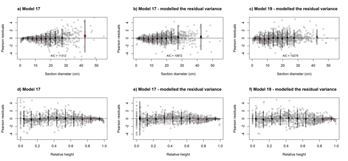
Fig. 4. Residuals plots for elaborated black locust fixed-effect taper model (Eq. 17, a, b, d, e) and mixed-effect taper model (Eq. 19, c, f) achieved for section diameter over bark according to the section diameter (upper part) and relative height (lower part). Grey dots define the Pearson residuals and large black dots show the means of the residuals in 10 classes of section diameter (upper part) and relative height (lower part). Thin vertical lines show the confidence interval of individual observations (mean ± 1.96 SD), and thick vertical lines (inside black dots) show the 95% confidence interval of the class mean. View larger in new window/tab.
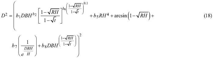
For the best model (Eq. 7) it was found that that for both section diameters (over and under bark) some of the estimated parameters are not statistically significant (b3, b6 and b7 for section diameter over bark and b3, b6 for section diameter under bark). Hence, the selected best taper model (Eq. 7) for section diameter over bark was:
and for section diameter under bark was:
3.2 Section diameter – mixed-effects taper model
The taper model (Eq. 7), as the best fitted to the data, was also elaborated for section diameter over and under bark using a mixed-effects model approach. For section diameter over and under bark the lowest AIC value and the lack of convergence problems were achieved when three random parameters were defined (β1, β2, β3). In addition, it was possible to include between-tree variation in the lower, top, and middle parts of the stem (de-Miguel et al. 2012). Notwithstanding, evaluating the effect of the grouping level using the likelihood test revealed that in the case of section diameter over bark, random parameters should be defined not only on the tree, but also on the plot grouping level (p < 0.001, Table 4):
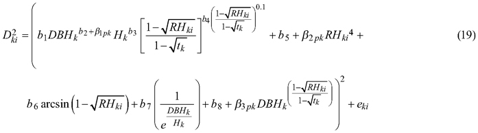
where p refers to the plot grouping level and k refers to the tree grouping level.
| Table 4. The parameter estimates and standard errors (in brackets) of the fixed-effects taper model (Eq. 17 and 18) and mixed-effects taper model (Eq. 19) for black locust. | |||||
| Parameter | Fixed-effects taper model | Mixed-effects taper model | |||
| section diameter over bark | section diameter under bark | section diameter over bark | section diameter under bark | ||
| b1 | 0.962 (0.026) | 0.629 (0.057) | –1.046 (0.105) | –0.917 (0.137) | |
| b2 | 0.983 (0.008) | 1.048 (0.023) | 0.926 (0.033) | 0.881 (0.072) | |
| b3 | - | - | 0.041 (0.031) | 0.081 (0.054) | |
| b4 | 0.289 (0.013) | 0.26 (0.015) | 0.262 (0.011) | 0.256 (0.009) | |
| b5 | –7.643 (0.763) | –7.565 (0.772) | 9.669 (1.031) | 9.483 (0.585) | |
| b6 | - | - | 2.944 (0.641) | 3.858 (0.547) | |
| b7 | - | 2.949 (0.67) | –2.041 (0.541) | –3.379 (0.814) | |
| b8 | 0.061 (0.005) | 0.047 (0.005) | –0.134 (0.017) | –0.142 (0.014) | |
| Plot level | sd(β1) | - | - | 0.009 | - |
| sd(β2) | - | - | 2.932 | - | |
| sd(β3) | - | - | 0.032 | - | |
| corr (β1, β2) | - | - | 0.520 | - | |
| corr (β1, β3) | - | - | 0.517 | - | |
| corr (β2, β3) | - | - | 1 | - | |
| Tree level | sd(β1) | - | - | 0.012 | 0.023 |
| sd(β2) | - | - | 0.722 | 1.911 | |
| sd(β3) | - | - | 0.056 | 0.061 | |
| corr (β1, β2) | - | - | 1 | 0.779 | |
| corr (β1, β3) | - | - | 1 | 0.781 | |
| corr (β2, β3) | - | - | 1 | 1 | |
| σ2 | - | - | 0.1152 | 0.0812 | |
| 1.345 | 1.331 | 1.843 | 1.823 | ||
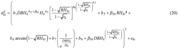
While for section diameter under bark the plot grouping level does not effect of the relationships among all groups of the dataset (p = 0.988, Table 4) and random parameters were defined for the tree grouping level only:
The analysis of the residuals for above models (Eq. 19 and 20) indicated the occurrence of heteroscedasticity. Therefore, as in case of fixed-effect models, we modelled the residual variance using a power function. Likelihood testing indicated that the variance function such that: var(eki) = σ2DBHk2δ, where σ2 and δ are the estimated scale and shape parameters for the power function, respectively, has a significant influence on the model fit (p < 0.001, Figs. 4c and 4f, Table 4).
3.3 Over bark tree volume
The comparison of the predicted over bark tree volume based on the elaborated fixed
(Eq. 17) and mixed-effects taper models (Eq. 19) to the reference volume (Eq. 11) revealed that the obtained values were similar. A high correlation coefficient between the predicted and measured volumes was achieved both: for the fixed-effects model (0.995) and the mixed-effects approach (0.9951, Fig. 5).
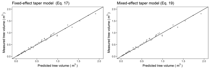
Fig. 5. Relationship between the reference (true) tree volume and predicted tree volume using the fixed-effects taper model (Eq. 17, left) and mixed-effects taper model (Eq. 19, right) for black locust.
The fixed-effects taper model (Eq. 17) was characterized by the narrowest 95% confidence interval achieved for the relative error (closely followed by the mixed-effect taper model, Eq. 19, Fig. 6). Among all analysed methods of determining the volume, equation (12) had the widest confidence interval for the relative error and significantly different from other models (Fig. 6).
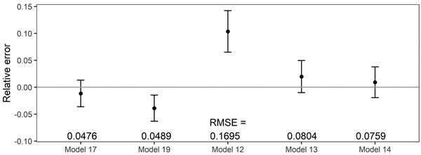
Fig. 6. 95% confidence intervals for the relative errors achieved during volume prediction based on all analysed volume equations for black locust. Model 17 – fixed-effects taper model (Eq. 17), Model 19 – mixed-effects taper model (Eq. 19), Model 12 – Moshki and Lamersdorf 2011 (Eq. 12), Model 13 – Sopp and Kolozs 2000 (Eq. 13), Model 14 – Lockow and Lockow 2015 (Eq. 14).
The lowest root mean square error for volume prediction (0.0476 m3) was obtained for the elaborated fixed-effect taper model (Eq. 17, Fig. 6). In the case of the mixed-effect taper model, this error was slightly larger and amounted to 0.0489 m3. Other available equations for black locust allow the prediction of volume with a larger root mean square error – the largest (0.1695 m3) in the case of equation (12, Fig. 6).
4 Discussion and conclusions
The elaborated taper models make it possible to obtain the section diameters (at any point on a stem) over and under bark. The goodness-of-fit measures indicated that taper model (Eq. 7) performed the best for both section diameters among all the analysed functions. The model required four independent variables: diameter at breast height over bark, tree height, relative height and relative breast height. In addition, this model included eight estimated parameters, which is the largest number analysed. The results indicate that the greater the number of estimated parameters is, the better the elaborated models fit to the data. In this case, however, for a small number of parameters, similar to the results by de-Miguel et al. (2012), this trend is not maintained. The results obtained indicate that the worst fitted model (Eq. 3) included three estimated parameters, and the models with two parameters (Eqs. 1 and 2) better described the shape of black locust than model (Eq. 3). Notwithstanding, as in the case of de-Miguel et al. (2012) research, not all estimated parameters of the best-fit model proved to be statistically significant. It is also worth mentioning the multicollinearity, which is defined as a high degree of correlation among independent variables (Rojo et al. 2005). Kozak (1997) claims that it does not substantially affect the predictive ability of the taper model. However, when defining random effects, model parsimony should also be considered (Cieszewski and Strub 2018).
The best fitted taper model (Eq. 7), similar to models (Eq. 5) and (Eq. 6), was defined as a variable-form function. Variable-form functions are simple continuous functions that describe the longitudinal stem shape with a varying exponent from base to top to account for neiloid, paraboloid and conic forms (Burkhart and Tomé 2012). Those types of taper models were first elaborated in British Columbia from 33 species groups (Kozak 1988), and these models are still evolving using different fitting methods (Socha et al. 2020). In addition, Zheng et al. (2017) indicated that variable taper equations can sometimes provide more flexible descriptions of tree profiles than simple taper equations, especially in the lower part of a stem. However, a disadvantage of variable-form taper equations is that they cannot be analytically integrated to calculate total stem or log volumes (Muhairwe 1999; Diéguez-Aranda et al. 2006). Moreover, Zheng et al. (2017) claimed that those taper models suffered from statistical complexity, resulting in difficulty in being understood and correctly used by forest managers.
The taper model (Eq. 7) was developed by Kozak based on data of western hemlock trees collected from Coastal British Columbia (Kozak 1997). It contains the constant relative breast height (t), and its exponent was created in such a way that the intercorrelations between the independent variables are low. De-Miguel et al. (2012) recognized Kozak’s model as being the best one among 33 analysed taper functions to predict the volume of Brutia pine (Pinus brutia Ten.). In addition, the authors evaluated the impact of individual estimated parameters on modelling the shape of the tree at different places on the stem. This information allows assessment of the impact of modifications to individual parameters e.g. when defining random effects.
Taper models can be elaborated for the use of the mixed-effects modelling approach. One of the main advantages of this solution is the possibility of implementing random effects during feature prediction, using a small amount of additional measurements in a plot (Pinheiro and Bates 2013; Bronisz and Mehtätalo 2020). In this context, Arias-Rodil et al. (2015) indicated that additional section diameters measured between 40% and 60% of the total tree height showed the greatest improvement in volume and diameter predictions. However, obtaining additional measurements, i.e., section diameters (especially under bark), is troublesome in practice. One of the possibilities of potentially using the mixed-effects modelling approach is the possibility of non-invasively obtaining additional data for the prediction of random effects using laser dendrometers (Cao and Wang 2011). Another option, which allows the prediction of random effects without additional measures, is computing the mean predictions from a mixed-effects model over the distribution of random effects (de-Miguel et al. 2012). However, to determine a solution that is simple to use in practice, fixed-effects predictions under the assumption that the random effects equal zero remains.
In the case of our research, the use of elaborated fixed-effect taper model (Eq. 17) better described the section diameter, which translates into more accurate volume prediction than fixed effects of the elaborated mixed-effects taper models (Eq. 19). Similar to our results, Arias-Rodil et al. (2015) or Pukkala et al. (2019) claim that if additional diameter measurements are not available, the fixed-effects modelling approach exhibits an advantage for tree volume prediction. Moreover, de-Miguel et al. (2012) points to another possibility. Assessing three prediction strategies for taper model elaborated by Kozak (Eq. 7, Kozak 1997) authors claim that strategy 3, calculating a marginal prediction based on the mixed-effects model by averaging the predictions over the estimated distribution of random effects, is recommendable for practical use in volume prediction.
In general, mixed-effect models are used mainly for two reasons: (i) to take into account the dependence of observations from some groups and (ii) to allow group-level prediction. Having regard to the above aspects, during our analyses we took into account two grouping levels: tree level and plot level (Lappi 1986). It turned out that only in the case of diameter over bark considering both grouping levels to create two-level mixed-effect model is beneficial (Eq. 19). Whereas Arias-Rodil et al. (2015), analysing both grouping levels, points that tree level explained much more variability in data than the plot level which reflects in our results on diameter under bark.
One of the main purposes of the elaborated taper models is the ability to predict the volume of trees (Burkhart and Tomé 2012). These models are valuable alternatives to the formulas developed using the DBH and tree height as independent variables (e.g., Eqs. 12–14). Likewise, the difference between the volume REs achieved based on the elaborated taper models (Eqs. 17 and 19) does not differ significantly from the results obtained for different volume equations available for black locust (e.g. Eq. 14). Model (Eq. 14) was developed in Brandenburg (eastern part of Germany) and was the basis for the development of German volume tables for black locust (Lockow and Lockow 2015). It can be assumed that one of the reasons for the similarities obtained is the close location of the sample plots to the data collection locations used by the German authors. Despite the lack of differences in the volume prediction errors, the advantage of taper models lies in the fact that they can be used to predict the section diameter or volume of any part of the stem (Kozak et al. 1969) and, as a result, they can be used to obtain the volumes of any product possible to be made from the harvested timber.
Acknowledgements
The research was financed by (i) the General Directorate of State Forests research grant: “Ecological and economic consequences of the selected alien tree species silviculture in Poland”, and (ii) Warsaw University of Life Sciences-SGGW internal scholarship fund.
References
Arias-Rodil M., Castedo-DoradoF., Cámara-Obregón A., Diéguez-Aranda U. (2015). Fitting and calibrating a multilevel mixed-effects stem taper model for maritime pine in NW Spain. PLOS ONE 10(12) article e0143521. https://doi.org/10.1371/journal.pone.0143521.
Bi H. (2000). Trigonometric variable-form taper equations for Australian eucalypts. Forest Science 46(3): 397–409.
Biging G.S. (1984). Taper equations for second-growth mixed conifers of northern California. Forest Science 30(4): 1103–1117.
Bolat I., Kara Ö., Sensoy H., Yüksel K. (2015). Influences of Black Locust (Robinia pseudoacacia L.) afforestation on soil microbial biomass and activity. IForest – Biogeosciences and Forestry 9(1): 171–177. https://doi.org/10.3832/ifor1410-007.
Bronisz K., Mehtätalo L. (2020). Mixed-effects generalized height–diameter model for young silver birch stands on post-agricultural lands. Forest Ecology and Management 460: 117901. https://doi.org/10.1016/j.foreco.2020.117901.
Bronisz K., Zasada M. (2019). Comparison of fixed- and mixed-effects approaches to taper modeling for Scots pine in west Poland. Forests 10(11) article 975. https://doi.org/10.3390/f10110975.
Brooks J.R., Jiang L., Clark A. (2007). Compatible stem taper, volume, and weight equations for young longleaf pine plantations in southwest Georgia. Southern Journal of Applied Forestry 31(4): 187–191. https://doi.org/10.1093/sjaf/31.4.187.
Bruce R., Curtiss L., and Van Coevering C. (1968). Development of a system of taper and volume tables for red alder. Forest Science 14: 339–350. https://doi.org/10.5962/bhl.title.87932.
Bruchwald A. (1980). Wykorzystanie badań nad pełnością strzał do budowy tablic zbieżystości dla drzewostanów sosnowych. [Using studies of stem form to establish tables of taper for Scots pine stands]. Folia Forestalia Polonica, A (Leśnictwo) 24: 101–109. [In Polish].
Burkhart H.E., Tomé M. (2012). Modeling forest trees and stands. Springer Dordrecht. 461 p. https://doi.org/10.1007/978-90-481-3170-9.
Cao Q.V., Wang J. (2011). Calibrating fixed- and mixed-effects taper equations. Forest Ecology and Management 262(4): 671–673. https://doi.org/10.1016/j.foreco.2011.04.039.
Cieszewski C.J., Strub M. (2018). Comparing properties of self-referencing models based on nonlinear-fixed-effects versus nonlinear-moixed-effects modeling approaches. Mathematical and Computational Forestry & Natural-Resource Sciences 10(2): 46–57.
de-Miguel S., Mehtätalo L., Shater Z., Kraid B., Pukkala T. (2012). Evaluating marginal and conditional predictions of taper models in the absence of calibration data. Canadian Journal of Forest Research 42(7): 1383–1394. https://doi.org/10.1139/x2012-090.
Demaerschalk J.P. (1972). Converting volume equations to compatible taper equations. Forest Science 18(3): 241–245. https://doi.org/10.1093/forestscience/18.3.241.
Diéguez-Aranda U., Castedo-Dorado F., Álvarez-González J.G., Rojo A. (2006). Compatible taper function for Scots pine plantations in northwestern Spain. Canadian Journal of Forest Research 36(5): 1190–1205. https://doi.org/10.1139/x06-008.
Dudzińska M. (2003). Model udziałów miąższości poszczególnych części strzały dla buka górskiego i nizinnego. [Model of the percentage of the stem section volume in the total stem volume for the mountain and lowland beech]. Sylwan 147(4): 28–37. https://doi.org/10.26202/sylwan.2003038. [In Polish].
Fowells H.A. (1965). Silvics of forest trees of The United States: agriculture handbook No. 271. U.S. Department of Agriculture. 762 p.
Horodecki P., Nowiński M., Jagodziński A.M. (2019). Advantages of mixed tree stands in restoration of upper soil layers on postmining sites: a five-year leaf litter decomposition experiment. Land Degradation & Development 30(1): 3–13. https://doi.org/10.1002/ldr.3194.
Jagodziński A.M., Wierzcholska S., Dyderski M.K., Horodecki P., Rusińska A., Gdula A.K., Kasprowicz M. (2018). Tree species effects on bryophyte guilds on a reclaimed post-mining site. Ecological Engineering 110: 117–127. https://doi.org/10.1016/j.ecoleng.2017.10.015.
Kozak A. (1988). A variable-exponent taper equation. Canadian Journal of Forest Research 18(11): 1363–1368. https://doi.org/10.1139/x88-213.
Kozak A. (1997). Effects of multicollinearity and autocorrelation on the variable-exponent taper functions. Canadian Journal of Forest Research 27(5): 619–629. https://doi.org/10.1139/x97-011.
Kozak A., Munro D.D., Smith J.H.G. (1969). Taper functions and their application in forest inventory. The Forestry Chronicle 45(4): 278–283. https://doi.org/10.5558/tfc45278-4.
Lappi J. (1986). Mixed linear models for analyzing and predicting stem form variation of Scots pine. Communicationes Instituti Forestalis Fenniae 134. 69 p. http://urn.fi/URN:ISBN:951-40-0731-X.
Lee W.-K., Seo J.-H., Son Y.-M., Lee K.-H., von Gadow K. (2003). Modeling stem profiles for Pinus densiflora in Korea. Forest Ecology and Management 172(1): 69–77. https://doi.org/10.1016/S0378-1127(02)00139-1.
Li G., Xu G., Guo K., Du S. (2014). Mapping the global potential geographical distribution of black locust (Robinia Pseudoacacia L.) using herbarium data and a maximum entropy model. Forests 5(11): 2773–2792. https://doi.org/10.3390/f5112773.
Lockow K.-W., Lockow J. (2015). Ertragstafel für die Robinie (Robinia pseudoacacia L.). [Yield tables for Black Locust (Robinia pseudoacacia L.)]. Cw Nordwestmedia Verlagsgesellschaft mbH. 38 p. [In German].
Max T.A., Burkhart H.E., (1976). Segmented polynomial regression applied to taper equations. Forest Science 22(3): 283–289.
Mehtätalo L., Lappi J. (2020). Forest biometrics with examples in R. Chapman & Hall/CRC, London, UK.
Moshki A., Lamersdorf N.P. (2011). Growth and nutrient status of introduced black locust (Robinia pseudoacacia L.) afforestation in arid and semi arid areas of Iran. Research Journal of Environmental Sciences 5(3): 259–268. https://doi.org/10.3923/rjes.2011.259.268.
Muhairwe C.K. (1999). Taper equations for Eucalyptus pilularis and Eucalyptus grandis for the north coast in New South Wales, Australia. Forest Ecology and Management 113 (2–3): 251–269. https://doi.org/10.1016/S0378-1127(98)00431-9.
Munro D.D. (1966). The distribution of log size and volume within trees. A preliminary investigation. Faculty of Forestry, University of British Columbia.
Nadal-Sala D., Hartig F., Gracia C.A., Sabaté S. (2019). Global warming likely to enhance black locust (Robinia pseudoacacia L.) growth in a Mediterranean riparian forest. Forest Ecology and Management 449 article 117448. https://doi.org/10.1016/j.foreco.2019.117448.
Newberry J.D., Burkhart H.E. (1986). Variable-form stem profile models for loblolly pine. Canadian Journal of Forest Research 16(1): 109–114. https://doi.org/10.1139/x86-018.
Nowiński M. (1977). Dzieje roślin i upraw ogrodniczych. [History of plants and horticultural crops]. PWRiL, Warsaw. 368 p. [In Polish].
Pinheiro J., Bates D. (2013). Mixed-effects models in S and S-PLUS. Springer-Verlag New York Inc. 528 p.
Pinheiro J., Bates D., Saikat D., Deepayan S. (2020). nlme: linear and nonlinear mixed effects models. https://cran.r-project.org/web/packages/nlme. [Cited 4 March 2020].
Pukkala T., Hanssen K.H., Andreassen K. (2019). Stem taper and bark functions for Norway spruce in Norway. Silva Fennica 53(3) article 10187. 15 p. https://doi.org/10.14214/sf.10187.
R Core Team (2020). R: a language and environment for statistical computing. R Foundation for Statistical Computing, Vienna, Austria.
Radtke A., Ambraß S., Zerbe S., Tonon G., Fontana V., Ammer C. (2013). Traditional coppice forest management drives the invasion of Ailanthus altissima and Robinia pseudoacacia into deciduous forests. Forest Ecology and Management 291: 308–317. https://doi.org/10.1016/j.foreco.2012.11.022.
Rédei K., Csiha I., Keserű Z., Végh Á.K., Győr J. (2012). The silviculture of black locust (Robinia pseudoacacia L.) in Hungary: a review. SEEFOR South-East European Forestry 2(2): 101–107. https://doi.org/10.15177/seefor.11-11.
Riemer T., von Gadow K., Sloboda B. (1995). Ein Modell zur Beschreibung von Baumschäften. [A model for describing tree stems]. Allgemeine Forst- und Jagdzeitung 166(7): 144–147. [In German].
Rojo A., Perales X., Sánchez-Rodríguez F., Álvarez-González J.G., von Gadow K. (2005). Stem taper functions for maritime pine (Pinus pinaster Ait.) in Galicia (Northwestern Spain). European Journal of Forest Research 124: 177–186. https://doi.org/10.1007/s10342-005-0066-6.
RStudio team (2015). RStudio: integrated development for R. RStudio Inc., Boston, MA.
Socha J. (2002). A taper model for Norway spruce (Picea abies (L.) Karst.). Electronic Journal of Polish Agricultural Universities. Series: Forestry 5(2).
Socha J., Kubik I. (2005). Model zbieżystości strzał dla górskich drzewostanów świerkowych średnich klas wieku. [Taper model for mountain spruce stands in medium age classes]. Sylwan 149(1): 42–52. https://doi.org/10.26202/sylwan.9200414. [In Polish].
Socha J., Netzel P., Cywicka D. (2020). Stem taper approximation by artificial neural network and a regression set models. Forests 11(1) article 79. https://doi.org/10.3390/f11010079.
Sopp L., Kolozs L. (2000). Wood volume tables. Agricultural Publishing House, Budapest.
Tokarska-Guzik B. (2005). The establishment and spread of alien plant species (Kenophytes) in the flora of Poland. Wydawnictwo Uniwersytetu Śląskiego.
Vítková M., Müllerová J., Sádlo J., Pergl J., Pyšek P. (2017). Black locust (Robinia Pseudoacacia) beloved and despised: a story of an invasive tree in Central Europe. Forest Ecolgy and Management 384: 287–302. https://doi.org/10.1016/j.foreco.2016.10.057.
Wickham H. (2016). ggplot2 – elegant graphics for data analysis. Springer, New York. 253 p. https://doi.org/10.1007/978-3-319-24277-4.
Wojda T., Klisz M., Jastrzębowski Sz., Mionskowski M., Szyp-Borowska I., Szczygieł K., (2015). The geographical distribution of the black locust (Robinia Pseudoacacia L.) in Poland and its role on non-forest land. Papers on Global Change 22: 101–113. https://doi.org/10.1515/igbp-2015-0018.
Womer R.B. (2012). The viability of black locust and the triakonta connection system as structural components in modular framing systems.
Yang Y., Huang S., Trincado G., Meng S.X. (2009). Nonlinear mixed-effects modeling of variable-exponent taper equations for lodgepole pine in Alberta, Canada. European Journal of Forest Research 128: 415–429. https://doi.org/10.1007/s10342-009-0286-2.
Yüksek T. (2012). The restoration effects of black locust (Robinia pseudoacacia L.) plantation on surface soil properties and carbon sequestration on lower hillslopes in the semi-humid region of Coruh Drainage Basin in Turkey. CATENA 90: 18–25. https://doi.org/10.1016/j.catena.2011.10.001.
Zheng C., Wang Y., Jia L., Mason E.G., We S., Sun C., Duan J. (2017). Compatible taper-volume models of Quercus variabilis Blume forests in north China. iForest – Biogeosciences and Forestry.10(3): 567–575. https://doi.org/10.3832/ifor2114-010.
Total of 55 references.
