Kalle Karttunen  ,
Lauri Lättilä,
Olli-Jussi Korpinen,
Tapio Ranta
,
Lauri Lättilä,
Olli-Jussi Korpinen,
Tapio Ranta
Cost-efficiency of intermodal container supply chain for forest chips
Karttunen K., Lättilä L., Korpinen O.-J., Ranta T. (2013). Cost-efficiency of intermodal container supply chain for forest chips. Silva Fennica vol. 47 no. 4 article id 1047. https://doi.org/10.14214/sf.1047
Highlights
- The combined availability and simulation study method obtains more realistic results for use in practical decision-making in supply chain management
- The total costs of forest chips with intermodal composite container supply chains were lower than traditional options in all scenarios
- The most advantageous way to expand the procurement area for forest chips is either to use composite container trucks or start using train transportation instead of trucks for procurement from longer distances.
Abstract
Cost-efficient solutions of supply chains for energy wood are required as part of endeavors to reach targets for renewable energy utilization. Long-distance railway transportation is an interesting area of research, especially for high-volume sites where the forest-to-site distance is considerable and rail facilities already exist. The aim of the study was to compare the cost-efficiency of an intermodal container supply chain and traditional multi-modal supply chain with corresponding direct truck logistics for long-distance transportation of forest chips. In the study, site-dependent information for forest biomass transport was integrated into a simulation model to calculate the cost-efficiency of logistic operations related to forest chips transportation in central Finland. The model was tested with several truck and railway transportation scenarios for varying demand of forest chips at the case power plant. The total costs of traditional supply chains were found to be 5–19% more expensive than container supply chain scenarios. The total unit costs of forest chips varied between 15.3 and 20.0 €/MWh depending on the scenario. It is concluded on the basis of the scenario study that intermodal light-structure container logistics and railway transportation could be developed as a viable option for large-scale supply of forest chips.
Keywords
trucks;
railways;
wood fuels;
transportation systems
-
Karttunen,
Lappeenranta University of Technology, LUT Savo Sustainable Technologies, Sammonkatu 12, FI-50130 Mikkeli, Finland
E-mail
kalle.karttunen@lut.fi
- Lättilä, Lappeenranta University of Technology, LUT Savo Sustainable Technologies, Sammonkatu 12, FI-50130 Mikkeli, Finland E-mail lauri.lattila@lut.fi
- Korpinen, Lappeenranta University of Technology, LUT Savo Sustainable Technologies, Sammonkatu 12, FI-50130 Mikkeli, Finland E-mail olli-jussi.korpinen@lut.fi
- Ranta, Lappeenranta University of Technology, LUT Savo Sustainable Technologies, Sammonkatu 12, FI-50130 Mikkeli, Finland E-mail tapio.ranta@lut.fi
Received 6 May 2013 Accepted 18 October 2013 Published 25 November 2013
Views 191737
Available at https://doi.org/10.14214/sf.1047 | Download PDF

1 Introduction
1.1 Background
Regional site-dependent features must be taken into account and incorporated into decision-making when building up a future bio-based economic system. Finland, situated in the northern boreal forest zone, is one of the world’s most heavily forested countries with forest coverage of 73% (United Nations 2012) and forests are the country’s biggest source of renewable energy. Alongside industrial use of roundwood, recent years have seen increased use of forest-based energy, particularly untreated chips straight from the forest (i.e. forest chips). This business area exhibits great potential for sustainable growth. The Finnish forest industry is currently facing problems in many of its core areas: weakening of export markets as a result of the global economic slump, structural changes in communication paper markets and increasing competition in the supply of paper and board products (Hetemäki and Hänninen 2009). In addition to the current economic problems, in the long term, ecological changes resulting from climate change induced by greenhouse gas emissions pose a further threat (IPCC 2007). Bioenergy will foreseeably play a key-role in reducing global greenhouse gas emissions in the long term (Chum et al. 2011) and the increased use of bioenergy creates opportunities for sustainably managed forests. Greater utilization of forest-based biomass for energy production may offer business opportunities not only for international forest and energy companies but also for local logistics companies and forest owners.
During the last decade, there has been a boom in the use of forest fuels for energy in Finland. Forest fuel is produced straight from the forest biomass, which is defined as the accumulated mass, above and below ground, of the wood, bark and leaves of tree species. Forest biomass utilized for energy purposes can be produced from logging residues, small-diameter energy wood, stumps and stem deadwood by chipping or crushing the wood into smaller chips. In 2011, 7.5 million cubic metres of forest chips were used for energy production, accounting for 13.7 TWh, or about 3.5%, of the country’s total energy use (Ylitalo 2012). The target for the end of 2020 has been set at 13.5 million cubic metres (Ministry of Employment and the Economy 2010).
A key challenge for forest fuels has been to utilize biomass volumes in an economical way. Availability and supply costs of forest fuels are very sensitive to worksite factors and transport distances (Ranta 2002). The main reason for high transport costs is the low energy density of forest fuels, which varies between 0.42 MWh/m3 (uncomminuted logging residues) and 0.81 MWh/m3 (chipped forest biomass) depending on the processed biomass material (Ranta and Rinne 2006). Measured on a regional basis, the potential demand for wood fuels for energy use is higher than the supply in all provinces of Finland, which increases the distances of forest fuel transportation (Ranta et al. 2007).
1.2 Long-distance transportation for forest biomass
For shorter distances (< 60 km), truck transportation of loose residues and end-facility comminution has hitherto been the most cost-competitive method (Tahvanainen and Anttila 2011) but over longer distances, roadside chipping with chip truck transport has been shown to be more cost-efficient (Ranta and Rinne 2006). For even longer distances (135–165 km), depending on the biomass source, train transportation of forest chips can offer the lowest costs when used in conjunction with roadside chipping systems (Tahvanainen and Anttila 2011). Inland barge transportation has also been studied and results indicate that barge transportation of roadside-chipped chips is more cost-efficient than truck transportation for distances greater than 100–150 km (Karttunen et al. 2012a).
Within the Finnish national context, especially the use of small-diameter energy wood could be increased to reach energy targets. More dense forest management of young stands, including energy wood thinning, can be used to produce small-diameter trees more economically (Heikkilä et al. 2009). Logging is the most expensive part of the supply chain for small-diameter energy wood (Laitila 2008) and the costs are significantly higher than those of logging residues (Hakkila 2004). Innovations leading to more efficient logging have been developed in recent years, such as single-grip harvester heads equipped with multi-tree handling equipment for cutting whole trees and multi-stem delimbed energy wood (Laitila et al. 2010a; Belbo 2011; Kärhä 2011). Other costs of the supply chain, such as chipping and transportation of chips, are quite similar for both small-diameter trees and logging residues (Laitila 2008; Hakkila 2004).
The most frequently used chipping method is roadside chipping, producing 50–60% of all forest biomass at the end of the twentieth century (Strandström 2013). Logging residues and small-diameter trees are mostly chipped at the roadside (70–80% share). Forest fuels are transported mainly by trucks to the power plants. Traditionally, a solid-frame ordinary trailer truck system is the most commonly used vehicle for peat and wood-chip transport logistics in Finland (Karttunen et al. 2012b). Typical frame capacities for ordinary trailers range between 120 and 140 m3 (66%) and tare weight of trucks between 20 and 25 tonnes (59%). The maximum weight limit in Finland for road transportation has recently changed from 60 tons to 64 tons for 7-axle vehicles for a trial period of 5 years. The maximum weight limit for 9-axle trucks has been increased to 76 tonnes and the maximum height from 4.2 to 4.4 metres.
Container trucks see marginal use (8%) in peat and wood-chip transport in Finland (Karttunen et al. 2012b). Three containers can be transported by a truck and ordinary trailer. The truck must feature a hook system to allow the transfer or unloading of the containers. Containers without doors need to be unloaded with a special turning machine. An innovative container made of composite material has been designed for intermodal truck and railway transportation (Ranta et al. 2011). The weight of the composite container is 1500 kg, half that of a traditional metal container. The composite container has been sized to allow a load of up to 20 tons. The container dimensions can be modified within the limits set by current road transport legislation (width 2.55 m, height 4.4 m, and length 25.25 m). To allow intermodal transportation, the container is designed to be suitable also for railway wagons. A watertight, thermally insulated structure prevents freezing-related problems in wintertime, which is a clear benefit in Nordic winter conditions (Föhr et al. 2013).
A current trend in the development of railway logistics has been to decrease the number of terminal sites (Iikkanen and Sirkiä 2011). From the point of view of the bio-based economy, the remaining sites should be better resourced, especially as regards biomass handling facilities. For example, container railway terminals need enough space for container-handling. At present, only part of the terminal network is suitable for container-handling of large quantities of forest biomass. Additionally, driving distances should be optimal to gain the advantages of rail-based transport from areas not normally used for forest fuel procurement.
The cost of railway transportation for hauling forest biomass in Finland has been simulated in an earlier study (Korpinen et al. 2011), where the average cost was 1.72 €/MWh (4.92 €/tn) with 15 wagons (distance 342 km). The simulation study indicated 10-wagon trains as more competitive than 20-wagon trains because of the lower utilisation rate of the latter. Korpinen et al. (2011) determined optimal wagon count via simulation and found that the significance of wagon count was rather low relative to the average costs if the train had seven or more wagons. Container railway logistics with terminals for wood fuels have been studied and taken into operational use in Sweden (Enström 2008; Enström and Winberg 2009).
Efficient supply chains for biomass are clearly of considerable significance for greater use of energy wood and thus form an interesting area of study. Specific issues that need addressing include: cost-efficient solutions for long-distance transportation – road, rail and combined approaches; cost structures of small-diameter energy wood, which unlike logging residues and stumps are not dependent on final cutting; and possible effects of new road dimensions and technical innovations such as intermodal containers, which are widely used in worldwide trade but have hitherto found little application in biomass transport.
1.3 Aim of the study
The aim of this study was to examine long-distance transportation of forest chips. The main focus of interest was determination of the profitability and competitiveness of an innovative intermodal composite container solution. The study compared a traditional multimodal supply chain with an intermodal container supply chain for long-distance transportation of wood chips by road and rail. The main difference between the supply chains is found in the functionality of the terminal operations: containers can be handled as individual units in the intermodal supply chain, whereas in traditional systems the chips must be unloaded and loaded as loose material. The study sought to address the question of whether utilization of intermodal composite containers could be a profitable and competitive transportation solution as a part of a large-scale forest biomass supply chain. Furthermore, the study evaluated in which situations it is worthwhile adopting an intermodal container supply chain for forest chips when the supply and demand of forest biomass resources are taken into account. The baseline of the study was a scenario of using truck transportation for forest chips around the user site for existing target demand.
A scenario comparison study method is utilized for the specific case of a selected power plant and composite container logistics. The case calculation is based on the demand of a modern combined heat and power (CHP) plant situated in Jyväskylä, Central Finland (62°11´N, 25°44´E). The CHP plant (power 370 MW) produces 240 MW district heat and 130 MW electricity using mainly wood and peat as fuel. The average annual use of forest fuels at the case plant has been over 500 GWh in recent years. There is potential for increasing the use of forest fuels, especially by activating the railway terminal and underused unloading facilities.
Availability of forest biomass resources to demand points has been studied using site-dependent information (Ranta 2002; Ranta 2004). In many studies, the costs of long-distance transportation for forest biomass have been determined using cost analysis, which has also been combined with availability analysis (Tahvanainen and Anttila 2011; Korpinen et al. 2013). The costs of long-distance forest biomass transportation have also been studied using a simulation method (Karttunen et al. 2012a; Korpinen et al. 2011).
This study contributes to the field by describing and evaluating a new solution for long-distance transportation of forest biomass. By extending analysis of the use of intermodal composite containers to forest biomass logistics, the study gives guidance to applications in which such systems could be adopted. The study introduces a combined methodology of availability analyses and a simulation method that permits the research problem to be addressed based not only on the site-dependent supply and demand potential but also on different transportation methods for forest biomass. By using combined methodologies, it is possible to obtain more realistic results for use in practical decision-making in supply chain management. The study increases understanding of potential methods for utilizing forest-based biomass resources for a more cost-efficient, sustainable and climate friendly energy future.
2 Material and methods
2.1 Study scenarios
This study comprises three main scenarios based on the chosen demand and supply chain. The main scenarios are divided into truck and railway transport options. The first scenario (Sce. 1) involves a comparison between intermodal container logistics and traditional solid-frame truck logistics for the estimated forest chips use at the case power plant. The second scenario (Sce. 2) considers similar truck transportation but with higher demand for forest chips and therefore longer distances. The third scenario (Sce. 3) considers the higher demand and longer distances together with the use of a railway supply chain in addition to the truck logistics. The sub-scenarios of the study compare the traditional and container supply chain options for both past and current maximum road transport dimensions. Additional scenarios for current dimensions are included in the simulation study. The scenarios are described in Fig. 1 and Table 1.
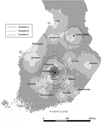
Fig. 1. Study area around the city of Jyväskylä (Scenarios 1 & 2) and around the satellite terminal of Kontiomäki (Scenario 3).
| Table 1. Main and sub-scenarios used in the study. Past (max. 60 tonnes) and current (max. 64 tonnes) road transport dimensions for traditional and container supply chains were compared. Additional sub-scenarios for current dimensions treat alternative numbers of trucks and wagons. Main scenarios: Sce. 1 = current use, Sce. 2 = additional use (by truck), and Sce. 3 = additional use (by train). | |||
| Sub-scenarios | Main scenarios | ||
| Sce. 1 | Sce. 2 | Sce. 3 | |
| Traditional | |||
| Past dimensions | 1.1.1 | 2.1.1 | 3.1.1 |
| Current dimensions | 1.1.2 | 2.1.2 | 3.1.2 |
| a. Sub-scenario | 1.1.3 | 2.1.2 | 3.1.3 |
| b. Sub-scenario | 3.1.4 | ||
| Container | |||
| Past dimensions | 1.2.1 | 2.2.1 | 3.2.1 |
| Current dimensions | 1.2.2 | 2.2.2 | 3.2.2 |
| a. Sub-scenario | 1.2.3 | 2.2.3 | 3.2.3 |
| b. Sub-scenario | 3.2.4 | ||
The demand and supply scenarios are limited to the forest based biomass of logging residues from final cuttings and small-diameter whole trees from early thinnings. The target demand for logging residues was kept lower and small-diameter trees higher in additional use of Sce. 2 compared to Sce. 3 (Table 2). The scenario volumes were chosen based on the current and potential additional demand of the case CHP plant and estimated according to the competition situation for each forest biomass source (Korpinen et al. 2012). Forest biomass (logging residues and small-diameter energy wood) stored at the roadside forms the starting point of the simulation and is the point at which chipping and long-distance transport and other material-handling operations begin (Fig. 2).
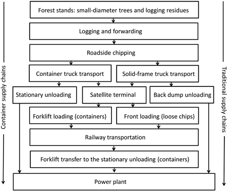
Fig. 2. Process description of material flows and handling operations of the supply chains studied.
| Table 2. Target demand of case power plant for forest chips (GWh). Sce. 1 = current use, Sce. 2 = additional use (by truck), and Sce. 3 = additional use (by train). | |||
| Biomass demand, GWh | |||
| Sce. 1 | Sce. 2 | Sce. 3 | |
| Base demand of Sce. 1 | - | 540 | 540 |
| Logging residues | 300 | 80 | 100 |
| Small-diameter trees | 240 | 120 | 100 |
| Total | 540 | 740 | 740 |
2.2 Availability analysis
The source data consisted of municipal estimates of forest fuel availability and land-use data (Korpinen et al. 2012). The datasets were imported to a geographical information system (GIS) environment that was processed by ArcGIS software (ESRI 2013).
The points of origin for forest-fuel supply were generated via a 4 × 4 km grid. The midpoints on the grid were extracted for further use in the transport analysis. This raster-to-vector conversion was required to connect the estimates of biomass availability to the transport network in vector format.
In practice, there may be several roadside sites in a 16 km2 area, and places of forest operations change from one year to the next as new cuttings appear. The biomass volumes in points closer than 4 km from one another were aggregated. Describing the information for several roadside sites as the attributes of one origin point decreases the computational load of route calculation.
The results of the availability analysis are given as average amounts of forest chips, including logging residues and small-diameter trees. Stumps were excluded from the study because they are normally chipped at terminal sites. The competitive demand for forest fuels was taken into account as market share analyses (Fig. 3) (Korpinen et al. 2012). Three zones were formed around each demand point separately for each fuel fraction and the total techno-economical biomass availability estimated for each zone. The zones were formed by connecting the closest origin points (by road) to the demand point until the total supply volume in the origin points meets the zone limit. The purpose of the rescaling is to relatively decrease the market shares of each demand point in the most competed areas where the sum of the theoretical market shares of the demand point exceeds 100%. The competitive demands for other large-scale biomass power plants were estimated similarly.
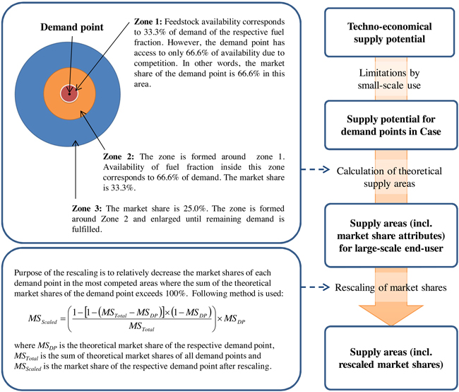
Fig. 3. Description of availability analysis for forest biomass in a competitive market (Korpinen et al. 2012).
The availability analysis gave results in solid-cubic meters, which were converted to megawatt hours using the following conversion factors. The dry density of whole trees was set at 430 kg/solid-m3 based on the average weight of birch and pine, whereas the logging residues of spruce were 445 kg/solid-m3 including half of the needles (Lindblad and Verkasalo 2001; Lindblad et al. 2010). The average moisture content for small-diameter energy wood (whole trees) was set to 40% and for logging residues to 45%, based on the average monthly delivery information of the case power plant in recent years. Average net calorific value was set to 19.3 MJ/kg for both biomass sources (Alakangas 2000). As a result, values of 10.60 MJ/kg (2.11 MWh/m3) for whole trees and 9.52 MJ/kg (2.14 MWh/m3) for logging residues were used for the purposes of calculation of the biomass availability in terms of energy value. The fixed moisture content was used in analysis of the average driving distances for the main scenarios. It must be noted that the moisture content and weight of the biomass was a variable factor in the simulation model of the transportation part of the supply chain. The simulation model used separate availability calculation with site-dependent information. The separate calculation method makes it possible to use the simulation model for other site-dependent case calculations.
2.3 Cost and efficiency analysis
The cost and efficiency analyses include all the cost structures and efficiency values of vehicles and machines throughout the supply chain from roadside to the power plant (Table 3). The supply chain must include all operations to get comparable results between traditional and container logistics. The operating costs (excluding VAT) of the alternative vehicles and machines were calculated with the aid of machine cost structure analysis and costs were presented in Euros (€). Machine cost structure analysis included annual fixed costs (e.g. capital depreciation, interest expenses, insurance fees and administration expenses) and variable operating costs (e.g. labor costs, fuel, repairs, service) which were set for the input values of the simulation model. The effective time (E0) productivities of vehicles and machines were converted to gross effective time productivities (E15), which included delays shorter than 15 min. The productivity times and the operating hour productivity coefficients were based on both estimates of the author and earlier follow-up or pre-test studies. The new approach and large number of alternatives meant that exact productivity information was not always available. Productivity estimates (unit/time) were converted into efficiency figures (time/unit) within minimum to maximum value ranges in the simulation timetable, where the delays and idle times were taken into account. The purchase prices and annual fixed costs of the trucks showed only slight differences and the variable costs of both types of trucks had the same unit costs, although the final costs varied with distance and net tonnes due to the payload difference of the vehicles.
| Table 3. Used purchase price and annual costs of machines and vehicles used in the simulation model. Prices and costs are presented without Value Added Tax (VAT, 0%). | |||
| Cost element | Purchased price, € | Annual fixed cost, €/a | Variable cost, €/unit |
| Truck transport (Sce. 1, 2 and 3) | |||
| Roadside chipper | 450 000 | 285 000 | 3 €/tn |
| Container truck | 270 000 | 83 000 | 0.012 €/tnkm |
| Unloading machine | 85 000 | 57 519 | 11.07 €/container |
| Solid-frame truck | 265 000 | 86 000 | 0.012 €/tnkm |
| Railway transport (Sce. 3) | |||
| Locomotive and wagons | 2 200 000 | 319 039 | |
| Intermodal composite container | 15 000 | 5400 | 0.016 €/tnkm |
| Metal container | 8390 | 3036 | 0.013 €/tnkm |
| Front-loader | 205 000 | 154 202 | - |
| Forklift loader | 250 000 | 179 023 | - |
| Unloading machine | 85 000 | 57 519 | 11.07 €/container |
The supply chains had similarities and differences depending on the chosen scenario. In train logistics (Sce. 3), a forklift loader and stationary unloading machine were used at the power plant terminal for unloading both intermodal composite and traditional metal containers. At the satellite terminal there were logistical differences; with the loading operations to be done either with a forklift loader for intermodal containers or traditionally with a front-loader for loose forest chips. There were also differences in daily chipping productivity because of payload capacity (Rinne 2010). At the roadside storage, the trucks had an assumption (5% probability) that the chipper would not be ready to start the chipping/loading operation and waiting time would last a maximum of 30 minutes per truck in the simulation model. The cost of a chipper was analysed using two trucks per chipper in the supply chain, and the average stationary-unloading cost included three trucks (nine containers). Profits of entrepreneurship were not taken into account in the cost structures and simulations.
The lifespan of the containers was set to 20 years. The vehicles were given different lifespans: 7 years for chippers and trucks, and 10 years for loaders. The calculation system of truck transportation is based on cost-structure parameters received from entrepreneurs, vehicle constructors and the road transport association, Finnish Transport and Logistics (SKAL). The study involves the difference between a solid-frame, i.e., a traditional truck, and a truck with intermodal containers, i.e., a container truck. The train system can be based on a multimodal system when traditional trucks are used and an intermodal system with container trucks. The typical solid-frame truck set-up used in the study had a 127 m3 load size and the tare weight of the truck was 25 tonnes. Consequently, the maximum payload was limited to 35 tonnes based on the Finnish road transport limitation of 60 tonnes in the scenarios for past road dimensions (Karttunen et al. 2012b). Correspondingly, the container truck had a 124 m3 load size and the tare weight of a truck with ordinary trailer and containers was 20 tonnes, so the maximum payload was 40 tonnes. Recently introduced maximum road vehicle dimensions increased the volume in height (20 cm, 7.5% more) and maximum payload (4 tons, 10–11% more) for both trucks. In the simulation model, the transported payload varied according to the moisture content of the forest chips (Fig. 4). The restrictive factor of the payload is either the weight limit, for transporting moist biomass, or the frame volume of the truck, for transporting dryer biomass (30–60%: 261–390 kg/loose-m3).
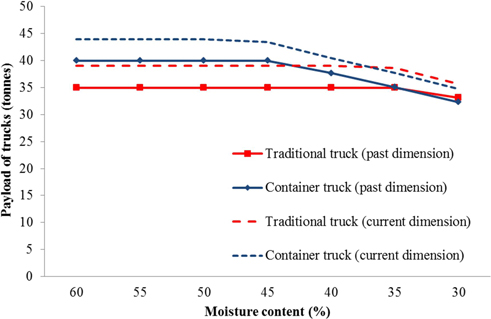
Fig. 4. Payload of forest chips (tonnes) for traditional trucks and container trucks based on past and current dimensions and the moisture content of forest chips.
The cost for railroad transport used in this study has originally been calculated from Swedish figures. The calculation tool, FLIS, created by Skogforsk, was used for calculation of the cost structures for rail transport (Table 4). Some adjustment to Finnish infrastructural fees has been made (Nash 2005). Kilometres were maintained constant (363 km) in this specific case from the Kontiomäki terminal to the power plant in Jyväskylä. 20 wagons per train (3 containers per wagon i.e. a total of 60 containers) were used for both intermodal composite containers (41.3 m3/container, 1500 kg/container) and metal containers (46 m3/container, 2900 kg/container) in the sub-scenarios. In some sub-scenarios 15 wagons were also tested.
| Table 4. Railway transportation cost structure components (%-share) as an example for intermodal composite and interchangeable metal containers. | |||
| %-share | Cost component | Metal containers | Intermodal composite containers |
| Fixed costs | Locomotive and wagons | 15 | 11 |
| Rail infra | 13 | 9 | |
| Containers | 16 | 36 | |
| Variable cost | Operational cost (363 km) | 40 | 33 |
| Gross tonne cost | 10 | 7 | |
| Maintenance | 5 | 4 | |
| Total cost | 100 a) | 100 a) | |
| a) Total annual cost of railway transportation (180 trips and 20 wagons) was 1 136 000 € for metal containers and 1 586 000 € for intermodal composite containers. | |||
In the simulation model, the intermodal composite containers were loaded and unloaded using a forklift loader. The metal containers were loaded with a wheeled front-loader, but unloading was arranged in the same way as the intermodal containers at the power plant, i.e., using a fork loader and stationary unloading machine next to the railway line. The parameters given in Table 5, which are based on earlier productivity estimates and demonstrations (Karttunen et al. 2010; Föhr et al. 2013), were used in the calculations.
| Table 5. Average efficiency (minutes/unit) of loading and unloading (Sce. 1, 2 and 3). | ||
| Transport option | Efficiency, minutes/unit | |
| Loading (min–max) | Unloading (min–max) | |
| Truck transport | ||
| Traditional truck | ||
| Sce. 1 and 2 | 50–80/truck | 25–35/truck |
| Sce. 3 (terminals) | 50–80/truck | 25–35/truck |
| Container truck | ||
| Sce. 1 and 2 | 50–80/truck | 8–10/container |
| Sce. 3 (terminals) | 50–80/truck | 4–6/container |
| Railway transport | ||
| Intermodal composite container | 1–3/container | 5–7/container |
| Metal container | 2–3/container | 5–7/container |
A special emptying system is required for containers without doors. The container unloading system can be based on stationary or movable solutions (Fig. 5). In all cases, a heavy forklift or wheel loader is needed in terminal actions to transfer containers from one vehicle to another. Containers can also be unloaded directly from trucks to the stationary unloading system without special machine. The cost of the forklift loader was not included in the operation costs of unloading in the main terminal of power plant in this study.
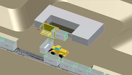
Fig. 5. Stationary unloading machine with forklift loader to transfer composite containers from a train (Fibrocom Ltd., Supercont®).
2.4 Simulation methodology
The simulation was conducted with AnyLogic 6 software, which is suitable for discrete-event and process-centric modelling (XJ Technologies 2013). The simulation model was constructed through a combination of agent-based modelling and discrete-event simulation. The model consists of a fixed number of truck agents and a final user-site and follows a discrete-event structure (Lättilä 2012). The train scenario was additionally created as an agent model but it followed the more complex discrete-event structure, including loading and unloading terminals.
The trucks have five distinct states: out of service, waiting, moving, being loaded, and emptying. The trucks are out of service as their schedules indicate between maximum 24:00 p.m. and minimum 7:00 a.m. on every weekday and are unused at weekends. The trucks operate in two shifts from November until April, and have one shift in May–June and September–October. The trucks do not operate during July–August. The trucks wait at the main terminal of the power plant until they have potential cargo. The state chart for the truck agents presented in Fig. 6 shows the logic of the trucks in the simulation model.
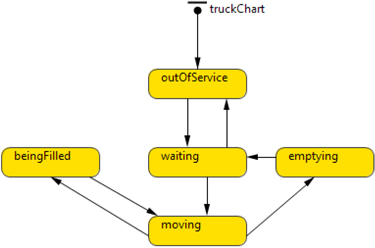
Fig. 6. State chart for the truck agents.
The cargo is generated according to the availability analysis. GIS data are used to estimate how long it takes a truck to drive to a potential load. There are 20 potential loads in the model at all times. The model checks beforehand if there is time to pick up and return any of the cargo loads according to the day schedule. When appropriate cargo is found, a truck moves to the location. The delay required for the move depends on the distance and the type of road between the terminal and the cargo location. When the truck reaches the location, it is loaded. During this time, the weight of the truck increases in accordance with the moisture level of the cargo. The weight of the load depends mainly on the moisture content of the forest chips, and the load is converted from tonnes to megawatt hours using conversion factors (Alakangas 2000). The moisture content of the forest chips ranges between 30% and 60% and is allocated to the simulation model according to the normal distribution for the chosen forest chip source. On completion of loading, the truck moves back to the terminal to be emptied. Next, the truck is commanded to seek for potential cargo and the route cycles are continued. At the end of the day, the truck returns to the ‘Out of Service’ state.
The simulation process description consists of input and output data for the chosen scenarios (Fig. 7). Time usage of the vehicles and unit costs for the chosen scenarios are the main output results of the simulation. The simulation model keeps track of the costs of the systems (Fig. 8). The model runs in the virtual reality for one year and calculates the total costs, which consist of the yearly fixed costs plus variable costs dependent on the production amount of forest chips. The total costs are then divided by the total amount of energy transported to the final user site, to yield the unit cost of energy as euros per megawatt hours. It is possible to stop the model during the year to analyse the total unit costs of other utilization rates.
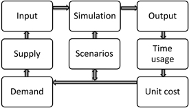
Fig. 7. Simulation process description consisting of input (supply and demand) and output (time usage and unit cost) data for chosen scenarios.
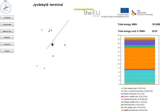
Fig. 8. Screen shot from the display of the simulation model used in the study.
In the simulation model, the train operates only in the wintertime when the trucks are operating two shifts because of high demand for forest chips. The train leaves the loading terminal (satellite terminal) in the early evening and the unloading terminal (main terminal of power plant) in the early morning. Thus, the train conducts four round-trips per week. A one-way trip takes approximately six hours, so there are six hours to load and another six hours to unload the train during a day. The state chart of the train is similar to the truck: the train is idle, moving between locations, or being loaded or unloaded.
The train can utilize different types of containers. If the train utilizes the same intermodal containers as the trucks, the truck operations at the loading terminal can be conducted using container trucks. The container trucks leave full containers at the terminal and pick up empty containers. At the satellite terminal, the train leaves empty containers and picks up full containers. A forklift loader conducts these operations for both the trucks and the train at the satellite terminal.
However, if larger containers are used on the train, traditional trucks are used to supply the terminal with the wood chips. The trucks empty their payload at the terminal and the railway wagons are loaded with a wheeled front loader. At the main terminal of the power plant, the same unloading machinery is assumed to be able to handle all of the different types of containers. The train is preferred over the trucks at the terminal. When the train arrives, the trucks have to wait for the train to be emptied before the unloading machinery starts to unload the trucks. This is due to the stricter time-constraints of the train, which has to follow a specific schedule.
2.5 Supply chain costs
Total costs of the supply chain include the many operations before long-distance transportation. These costs are the stumpage price for the forest owner, the harvesting costs (logging and forwarding) and operational overhead costs (organizational costs), which differ depending on the biomass source costs. In this study, the average logging cost (19.1 €/m3, 9.1 €/MWh) and the forwarding cost (5.6 €/m3, 2.7 €/MWh) for small-diameter energy wood (moisture content 40%) were based on earlier studies (Laitila 2008). An average piling cost of 0.5 €/m3, 0.2 €/MWh (Ranta 2002; Kärhä and Vartiamäki 2006) was used. The forwarding cost (6.2 €, 2.9 €/MWh) for loose logging residues (moisture content 45%) was based on previous studies (Laitila et al. 2010b; Asikainen et al. 2001). The overhead (organization of forest operation) and stumpage (payment to forest owners) costs were estimates (Heikkilä et al. 2009). The cost values used in the study are given in Table 6.
| Table 6. Roadside cost of logging residues and small-sized trees used in this study (€/MWh). | |||||
| Cost (€/MWh) | Overhead cost | Stumpage price | Logging cost | Forwarding cost | Total roadside cost |
| Logging residues | 0.5 | 0.5 | 0.2 | 2.9 | 4.1 |
| Small-diameter trees | 1.0 | 3.0 | 9.1 | 2.7 | 15.8 |
2.6 Assumptions and limitations
In this study, it was assumed that there is only one unloading station for forest chips in the power plant. Thus, the trucks need to wait for their unloading turn. In times of congestion during the peak season in winter, the waiting times would be longer than assumed in the simulation. The unloading times of the containers were based on a stationary unloading machine. Unloading times of the machine were based on pre-tests. Unloading of the train had to be done in the night or early morning because the container trucks, which were using the same unloading station in the simulation model, started the day schedule at 7 a.m. Different numbers of trucks were used in the simulation model to meet the target demand in the scenarios (Table 7).
| Table 7. Number of trucks used to fulfil the demand target of the scenarios in the simulation model. | ||||
| Number of trucks and wagons in the demand target of the scenarios | Sce. 1 (trucks) | Sce. 2 (trucks) | Sce. 3 (trucks) | (wagons) |
| Traditional truck | ||||
| Past dimensions | 10 | 18 | 14 | 20 |
| Current dimensions | 8 | 14 | 12 | 20 |
| a. Sub-scenario | 10 | 16 | 12 | 15 |
| b. Sub-scenario | 14 | 15 | ||
| Container truck | ||||
| Past dimensions | 8 | 12 | 12 | 20 |
| Current dimensions | 6 | 10 | 10 | 20 |
| a. Sub-scenario | 8 | 12 | 12 | 20 |
| b. Sub-scenario | 12 | 15 | ||
The container trucks and train were assumed to have another use during times of low demand for forest chips. For container trucks, the two summer months were free of costs. For the train, the costs included the costs for half a year, after which the train with the containers was considered as having another use. Totally, 45 extra containers were used in the intermodal supply chain.
Varying numbers of trucks and wagons (15 wagons = 45 containers) were included in the study of sub-scenarios dealing with current dimensions (Table 6). Truck and railway supply chain costs for current dimensions were put separately in the same figure to enable comparison of the cost-efficiency of the traditional supply chain with the container supply chain for alternative amount of forest chips for large-scale procurement from long distances. The aim of the additional sub-scenario analyses was to estimate combinations of trucks and wagons with the most potential to fulfill the need for forest chips cost-efficiently.
It is worth noticing that there is a difference between target demand and supply based on simulated deliveries in the study. Target demand is the aim of the power plant to fulfil its need for forest chips. Simulated supply is the volume of forest chips which it is possible to produce with the assumed number of vehicles based on simulation results. The unit cost of the supply chain is the result of the total costs divided by the simulated deliveries of forest chips.
3 Results
3.1 Total cost of the supply chain
Container supply chains were the most cost-efficient alternatives for both past (15.7–17.2 €/MWh) and current maximum truck dimensions (15.3–16.9 €/MWh) (Fig. 9). The past dimensions were 1–5% more expensive compared to the current dimensions. The unit costs of traditional supply chains varied between 17.0 €/MWh and 20.0 €/MWh for the past dimensions, which is 3–9% more expensive than with current dimensions (16.1 €/MWh–18.2 €/MWh), the precise amount depending on the scenario used. The total costs of the traditional supply chain were 8–19% greater than the corresponding container supply chain for the past dimensions and 5–11% greater for the current dimensions, depending on the scenario. The unit costs of truck and railway supply chains are presented separately (Fig. 10).
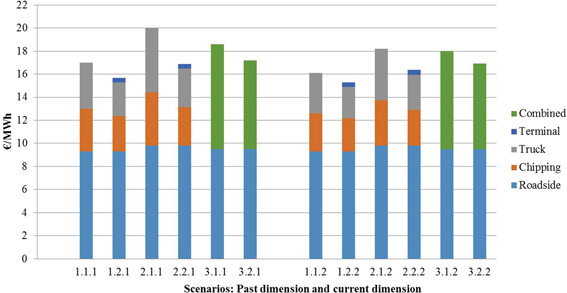
Fig. 9. Unit cost of forest chips (€/MWh) transported by traditional supply chain and container supply chain (past and current dimension). Combined system includes both truck and railway supply chains. Scenarios are presented in Table 1.
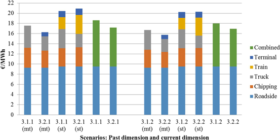
Fig. 10. Unit cost of forest chips (€/MWh) transported by traditional supply chain and container supply chain as calculated separately for the truck and railway supply chain (past and current dimension). Main terminal (around power plant) = mt; satellite terminal (around railway terminal) = st. Scenarios are presented in Table 1.
Total costs for current dimension scenarios (Table 8) varied between 7.4 and 14.7 million euros depending on the amount of forest chips (482–834 GWh) and logistical alternative (traditional or container supply chain). Unit cost varied between 15.3 and 20.0 €/MWh depending on the simulated amount of forest chips and logistical alternative. The unit cost of the railway supply chain varied between 20.3 and 26.5 €/MWh.
| Table 8. Simulated delivery and cost results of traditional and container supply chains for forest chips based on current dimension scenarios. Target demand results (200, 540 and 740 GWh/a) are also included. Scenarios are presented in Table 1. | |||||
| Scenarios | Delivery | Cost | |||
| Main scenarios | Sub-scenarios | Total, GWh/a | Railway, GWh/a | milj. €/a | €/MWh |
| Traditional | |||||
| Sce. 1 | 540 | 8.7 | 16.2 | ||
| 1.1.2 | 537 | 8.6 | 16.1 | ||
| 1.1.3 | 637 | 10.4 | 16.4 | ||
| Sce. 2 | 740 | 13.6 | 18.3 | ||
| 2.1.2 | 730 | 13.3 | 18.2 | ||
| 2.1.3 | 787 | 14.7 | 18.6 | ||
| Sce. 3 | 740 | 13.8 | 18.7 | ||
| 200 | (4.7) | (23.3) | |||
| 3.1.2 | 721 | 13.0 | 18.0 | ||
| 237 | (4.8) | (20.2) | |||
| 3.1.3 | 661 | 13.2 | 20.0 | ||
| 178 | (4.7) | (26.5) | |||
| 3.1.4 | 757 | 13.8 | 18.2 | ||
| 178 | (4.4) | (24.8) | |||
| Container | |||||
| Sce. 1 | 540 | 8.3 | 15.4 | ||
| 1.2.2 | 482 | 7.4 | 15.3 | ||
| 1.2.3 | 638 | 9.7 | 15.3 | ||
| Sce. 2 | 740 | 11.9 | 16.1 | ||
| 2.2.2 | 709 | 11.6 | 16.3 | ||
| 2.2.3 | 834 | 13.7 | 16.4 | ||
| Sce. 3 | 740 | 12.4 | 16.7 | ||
| 200 | (4.4) | (22.2) | |||
| 3.2.2 | 654 | 11.1 | 16.9 | ||
| 226 | (4.6) | (20.3) | |||
| 3.2.3 | 788 | 13.0 | 16.5 | ||
| 226 | (4.7) | (20.8) | |||
| 3.2.4 | 725 | 12.6 | 17.4 | ||
| 170 | (4.4) | (25.8) | |||
It is worth noticing that results of target demand (Main scenarios: 200, 540 or 740 GWh/a) are reported separately based on the cost curves for simulated delivery amounts of current dimensions (Table 8). Those simulations are included in the figures below, which present total cost of supply chains (Fig. 11, Fig. 12) and unit costs per MWh (Fig. 13, Fig. 14) separately for both the truck transportation and railway transportation chain.
The total cost curve (Fig. 11) shows that the cost curve of the traditional supply chain by trucks rises more steeply than the cost curve of the container supply chain as the amount of forest chips is increased, whereas the total cost curve of railway supply chains grows steadily (Fig. 12). Unit cost figures (Fig. 13, Fig. 14) show that the container supply chain is more cost-efficient than the traditional supply chain.
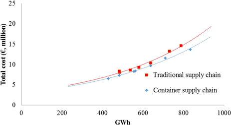
Fig. 11. Total cost (€, million) of traditional and container supply chains by trucks for forest chips (current dimensions).
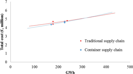
Fig. 12. Total cost (€, million) of traditional multimodal and container intermodal railway supply chains for forest chips (current dimensions).
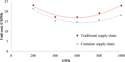
Fig. 13. Unit cost (€/MWh) of traditional and container supply chains by trucks for forest chips (current dimensions).
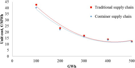
Fig. 14. Unit cost (€/MWh) of traditional multimodal and container intermodal railway supply chains for forest chips (current dimensions).
As an example, if deliveries of forest chips is increased from 600 GWh (average distance 71 km) to 800 GWh (95 km), the unit costs of the traditional supply chain by trucks increase from 17.2 to 19.2 €/MWh, whereas container supply chain costs by trucks increase from 14.7 to 15.8 €/MWh (Fig. 15). Consequently, savings potential grows exponentially from 1.5 to 2.7 €/MWh (annual savings from 0.9 to 2.2 million Euros) as a result of using the container supply chain instead of the traditional supply chain.
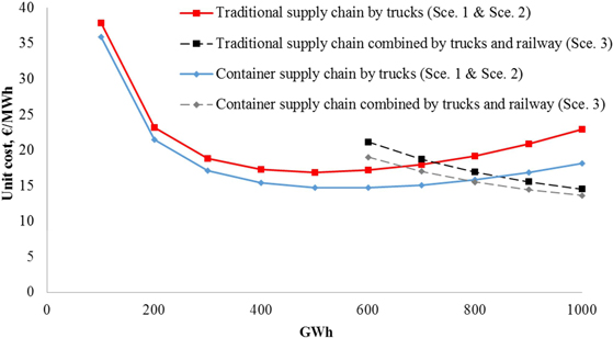
Fig. 15. Unit cost (€/MWh) of traditional and container supply chain scenarios for truck transportation (Sce. 1 & Sce. 2) and multimodal transportation (Sce. 3) for forest chips (current dimensions). The delivery amount of forest chips by trucks was kept constant (500 GWh) for multimodal supply chains (Sce. 3).
Combined multimodal truck and railway transportation (Sce. 3) can be used to decrease unit costs from longer distances (Fig. 15). For example, if the total deliveries of forest chips are increased from 600 to 800 GWh, so that the share of railway transportation is increased from 100 to 300 GWh, the unit costs of the traditional multimodal supply chain decrease from 21.2 to 16.9 €/MWh, whereas intermodal container supply chain costs decrease from 19.1 to 15.5 €/MWh. Savings potential cannot be achieved until the delivery amount of the railway supply chain is approaching 300 GWh, where the unit cost savings vary between 0.3 €/MWh (container) and 2.3 €/MWh (traditional) (annual savings from 0.2–2.3 million Euros) as a result of using railway system instead of trucks from long-distances.
3.2 Fixed and variable costs of truck transportation, chipping and unloading machine
The truck transportation unit cost for past maximum road vehicle dimensions was 4.0 €/MWh (1.1.1) for traditional trucks and 2.9 €/MWh (1.2.1) for container trucks (Sce. 1). Additional use of forest chips (Sce. 2) increased the truck transportation costs to 5.6 €/MWh (2.1.1) by traditional trucks and 3.3 €/MWh (2.2.1) by container trucks. Additional use of forest chips (Sce. 3) from the satellite terminal decreased the truck transportation cost, which was 4.2 €/MWh (3.1.1) for traditional trucks and 2.7 €/MWh (3.2.1) for container trucks, respectively. The costs of truck transportation with past dimensions were 7–28% more expensive than with current maximum truck dimensions, depending on the scenario. The simulated costs of the trucks, chipping and unloading machine are presented in Fig. 16.
The biggest costs of the transportation chain were the fixed costs of the trucks, which varied between 1.8 and 4.7 €/MWh depending on the scenario. The second biggest part was the fixed costs of chipping, which varied between 1.8 and 3.5 €/MWh.
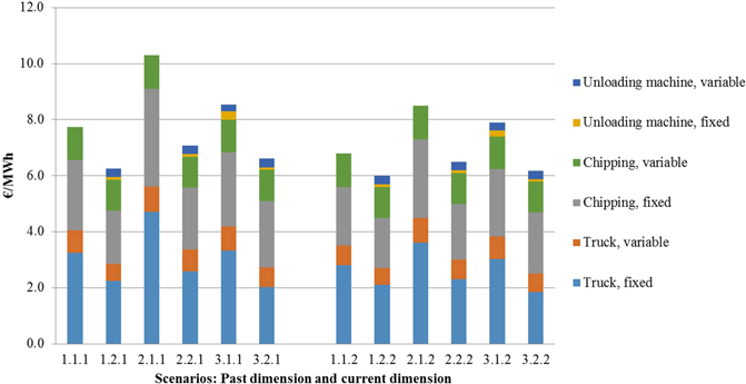
Fig. 16. Cost result (€/MWh) of simulation for truck transportation, chipping and the unloading machine in alternative scenarios (past and current dimension). Scenarios are presented in Table 1.
3.3 Simulated time usage of truck logistics
Simulated time usage of the truck logistics showed that the trucks stayed unused (“Trucks at base”) most (62–66%) of their annual time (Fig. 17). It is notable that the traditional trucks spend 14.8% of their time waiting to be emptied in the second scenario (2.1.1), which is clearly a bottleneck in traditional operations. For corresponding container trucks, the amount of waiting time remains low at 3.4% (2.2.1).
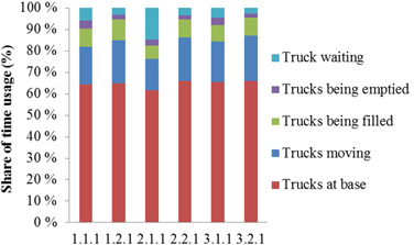
Fig. 17. Annual time usage of trucks in the scenarios (past dimension). Scenarios are presented in Table 1.
3.4 Average driving distances
The annual demand of Scenario 1 (Sce. 1) (540 GWh) was met within a 71 km average driving distance, which was two thirds of the longest driving distances (107 km) (Table 9). The average truck-driving distance has to be increased by 17% to 83 km to meet the additional demand of Sce. 2 (740 GWh). The average driving distance of Sce. 3 was the shortest, 65 km.
The low average driving distance of Sce. 3 was the result of the low driving distance around the satellite terminal, on average 48 km (maximum driving distance to the satellite terminal was 73 km) and average distances for the logging residues and small-diameter energy wood were 51 km and 46 km, respectively.
| Table 9. Average driving distances (in parentheses: maximum driving distance) by the trucks based on availability analysis for the target demand scenarios. | |||
| Distance, km | Sce. 1 | Sce. 2 | Sce. 3 |
| Logging residues | 61 (92) | 69 (103) | 59 (88) |
| Small-diameter energy wood | 81 (121) | 96 (144) | 71 (106) |
| Average | 71 (107) | 83 (124) | 65 (98) |
4 Discussion
This study determined and compared the cost of forest chips logistics for multimodal transportation supply chains based on traditional solid-frame options and intermodal containers. The results showed that the total costs of forest chips with intermodal composite container supply chains were lower than traditional options in all scenarios. The combined availability and simulation study method showed that the most advantageous way to expand the procurement area for forest chips is either to use composite container trucks or start using train transportation from longer distances.
Traditional systems were 8–19% more expensive (17.0–20.0 €/MWh) than the intermodal container scenarios (15.7–17.2 €/MWh) for past maximum road vehicle dimensions. Current dimension regulations decrease the total costs of forest chips by 0.2–1.9 €/MWh (on average 4%). The results for the intermodal container supply chain vary between 15.3 and 16.9 €/MWh, whereas traditional options were 5–11% more expensive (16.1–18.2 €/MWh) for current road vehicle dimensions. The change in road vehicle dimensions influenced traditional options more positively than container supply chains.
In order to increase the use of forest fuel at the power plant, it is necessary to increase the number of trucks. At the same time, a larger number of trucks leads to longer waiting times at the power plant level as it is difficult to effectively synchronize operations and trucks will arrive at the power plant at the same time. This creates a feedback with the required number of trucks because the trucks need to spend more of their operational time waiting at the unloading platform. For traditional trucks, it might be necessary to assess how to increase the number of slots for emptying at the power plant. Otherwise, increasing the driving distance will lead to non-linear increases in total costs of the logistics system as the number of required trucks is non-linear compared to the driving distance.
The availability analysis showed that it is possible to decrease truck driving distances dramatically if the additional procurement is extended via a railway satellite terminal with good biomass reserves rather than through direct truck hauling at the area of high demand and competition. On the other hand, additional handling and railway operations increased the total supply chain costs for the intermodal container supply chain more than direct truck hauling.
This study included a geographical information system (GIS) model combined with a simulation model to calculate the costs of a number of scenarios for the case area of Central Finland. A simulation method with many variable factors, such as payload differences, monthly demand of biomass, and including time usage of alternative machines should give more relevant cost results. Simulation study combined with geographical information will lead to results of greater relevance to practical decision-making when considering the use of innovations. A main difference between real prices and theoretical costs is the lack of profit cost data in the theoretical calculation scenarios. Moreover, in the scenarios, organizational overhead costs of transportation are not included in the total cost of the supply chain.
The unit costs of the railway transportation chain for forest chips varied between 2.2 and 3.7 €/MWh and total unit cost of the railway supply chain varied between 3.0 and 4.9 €/MWh, which included terminal costs of 0.8–1.2 €/MWh (loading and unloading). Intermodal container railway transportation was more expensive than traditional railway transportation, but combined supply chains of truck and railway transportation were more cost-competitive for intermodal container supply chains than traditional supply chains. The competitive market price of railway transportation could be more than theoretical costs, because profits were not included in the simulation. Not only combined methods of truck and railway supply chains but also combined methods of traditional and container supply chains might achieve optimal solutions for the large-scale supply chain of forest biomass.
It must be taken into consideration that this study included restrictions and assumptions that may have a significant role in supply chain costs. Firstly, it was assumed that there is only one unloading place for forest chips in the power plant. Container unloading times of the machine were based on pre-tests, but usability in real situations should be demonstrated to get more exact information about the productivity and functionality of the machine. Secondly, the container trucks and train were assumed to have another use during times of low demand for forest chips and fixed costs were excluded from the calculation. On the other hand, the cost of the traditional railway supply chain did not include summer seasons in the simulation model. The aim of the output settings of the supply chains was to maintain a good level of comparability for the study.
Thirdly, the payload is dependent not only on the biomass moisture content, tare weight and frame volume of the trucks but also on the road vehicle dimension limits by legislation. The vehicle dimension has an influence on costs, especially for wet and heavy forest chips. Light composite container trucks can take more payload than heavier traditional trucks. The Finnish government has decided to increase the maximum road transport limit in Finland from 60 tons to 76 tons. An increase to 64 tons for 7-axle trucks was used in this study, but 9-axle trucks can be driven with loads up to 76 tons. The use of container trucks for biomass transportation and usability of heavy volume traditional trucks with more axles are worthy of further investigation.
The case study showed that intermodal containers could be the most profitable alternative for forest biomass logistics. The results indicated that supply chain costs can be reduced by replacing traditional solid-frame transportation with the innovative intermodal container logistics or by replacing truck transportation with railway transportation for long distances. Intermodal composite container logistics and railway transportation could be developed as an attractive option for a large-scale supply chain for forest chips.
Acknowledgements
This study is based on the result of a project financed by the European Union (European Regional Development Fund) via Tekes, the Finnish Funding Agency for Technology and Innovation (EAKR, 2399/31/2010) and companies in the energy, forestry and logistics sector. We want to thank for all support. Special thanks to Johanna Enström, who helped with evaluation of railway costs using the FLIS calculation system created by Skogforsk.
References
Alakangas E. (2000). Suomessa käytettyjen polttoaineiden ominaisuuksia. [Properties of fuels used in Finland]. Valtion teknillinen tutkimuskeskus, VTT Tiedotteita – Research Notes 2045. [In Finnish].
Asikainen A., Ranta T., Laitila J. (2001). Hakkuutähdehakkeen kustannustekijät ja suurimittakaavainen hankinta. [Cost factors and large scale procurement of logging residue chips]. Research Notes 131. Faculty of Forestry, University of Joensuu. 107 p. [In Finnish].
Belbo H. (2011). Efficiency of accumulating felling heads and harvesting heads in mechanized thinning of small diameter trees. Linnaeus University Dissertations 66/2011.
Chum H., Faaij A., Moreira J., Berndes G., Dhamija P., Dong H., Gabrielle B., Goss Eng A., Lucht W., Mapako M., Masera Cerutti O., McIntyre T., Minowa T., Pingoud K. (2011). Bioenergy. In: Edenhofer O., Pichs-Madruga R., Sokona Y., Seyboth K., Matschoss P., Kadner S., Zwickel T., Eickemeier P., Hansen G., Schlömer S., von Stechow C. (eds.). IPCC special report on renewable energy sources and climate change mitigation. Cambridge University Press, Cambridge, United Kingdom and New York, NY, USA. http://dx.doi.org/10.1017/CBO9781139151153.006.
Enström J. (2008). Efficient handling of wood fuel within the railway system. In: Suadicani K., Talbot B. (eds.). The Nordic-Baltic conference on forest operations, Copenhagen, 23–25 September 2008. Forest and Landscape. Working Papers 30/2008. p. 53–55.
Enström J., Winberg P. (2009). Systemtransporter av skogsbränsle på järnväg. Arbetsrapport från Skogforsk 678. http://www.skogforsk.se/PageFiles/61310/Arbetsrapport%20678-2009.pdf.
ESRI (2013). http://www.esri.com/software/arcgis/. [Cited 1 June 2012].
Fibrocom Ltd. (2013). Supercont®. http://www.fibrocom.com/.
Föhr J., Karttunen K., Enström J., Johannesson T., Ranta T. (2013). Biomass freezing tests for composite and metal containers. 21st European Biomass Conference and Exhibition. Bella Center, Copenhagen, Denmark, 03–07 June 2013.
Hakkila P. (2004). Developing technology for large-scale production of forest chips. Wood Energy Technology Programme 1999–2003. Final report. National Technology Agency, Technology Programme Report 6/2004.
Heikkilä J., Sirén M., Ahtikoski A., Hynynen J., Sauvula T., Lehtonen M. (2009). Energy wood thinning as a part of the stand management of Scots pine and Norway spruce. Silva Fennica 43(1): 129–146.
Hetemäki L., Hänninen R. (2009). Arvio Suomen puunjalostuksen tuotannosta ja puunkäytöstä vuosina 2015 ja 2020. English summary and conclusions: Outlook for Finland’s forest industry production and wood consumption for 2015 and 2020. Metlan työraportteja 122. http://www.metla.fi/julkaisut/workingpapers/2009/mwp122.htm.
Iikkanen P., Sirkiä A. (2011). Development of the railway raw wood terminal and loading point network. Study covering all forms of transport. Research Reports of the Finnish Transport Agency 31/2011. ISBN 978-952-255-687-5.
IPCC (2007). Climate change 2007: synthesis report. Contribution of Working Groups I, II and III to the Fourth Assessment Report of the Intergovernmental Panel on Climate Change. IPCC, Geneva, Switzerland.
Kärhä K. (2011). Integrated harvesting of energy wood and pulpwood in first thinnings using the two-pile cutting method. Biomass and Bioenergy 35(8): 3397–3403. http://dx.doi.org/10.1016/j.biombioe.2010.10.029.
Kärhä K., Vartiamäki T. (2006). Productivity and costs of slash bundling in Nordic conditions. Biomass and Bioenergy 30(12): 1043–1052. http://dx.doi.org/10.1016/j.biombioe.2005.12.020.
Karttunen K., Föhr J., Ranta T. (2010). Energiapuuta Etelä-Savosta [Energywood from South-Savo]. Lappeenranta University of Technology, Faculty of Technology, Energy Technology, Reseach Report 7. [In Finnish].
Karttunen K., Väätäinen K., Asikainen A., Ranta T. (2012a). The operational efficiency of waterway transport of forest chips on Finland’s Lake Saimaa. Silva Fennica 46(3): 395–413.
Karttunen K., Föhr J., Ranta T., Palojärvi K., Korpilahti A. (2012b). Puupolttoaineiden ja poltto-turpeen kuljetuskalusto 2010. [Transportation vehicles for wood fuels and peat in 2010]. Metsätehon tuloskalvosarja 2/2012. ISBN 978-952-265-003-0. [In Finnish].
Korpinen, O-J., Jäppinen E., Ranta T. (2012). Advanced GIS-based model for estimating power plant’s supply logistics in a region with intense competition of forest fuel. World Bioenergy 2012, 29–31 May 2012, Jönköping, Sweden. World Bioenergy Proceedings. ISBN 978-91-977624-5-8.
Korpinen, O-J., Jäppinen E., Ranta T. (2013). Geographical origin-destination model designed for cost-calculations of multimodal forest fuel transportation. Journal of Geographical Information Systems 5(1). http://dx.doi.org/10.4236/jgis.2013.51010.
Korpinen, O-J., Föhr J., Saranen J., Väätäinen K., Ranta T. (2011). Biopolttoaineiden saatavuus ja hankintalogistiikka Kaakkois-Suomessa. [Availability and supply logistics of biofuels in Southeastern Finland]. Lappeenranta University of Technology, Faculty of Technology, LUT Energy, Research Report 12. [In Finnish].
Laitila J. (2008). Harvesting technology and the cost of fuel chips from early thinnings. Silva Fennica 42(2): 267–283.
Laitila J., Heikkilä J., Anttila P. (2010a). Harvesting alternatives, accumulation and procurement cost of small-diameter thinning wood for fuel in Central-Finland. Silva Fennica 44(3): 465–480.
Laitila J., Leinonen A., Flyktman M., Virkkunen M., Asikainen A. (2010b). Metsähakkeen hankinta- ja toimituslogistiikan haasteet ja kehittämistarpeet. [Challenges and development needs for the supply chain of forest chips]. VTT Tiedotteita – Research Notes 2564. [In Finnish].
Lättilä L. (2012). Improving strategic decision-making with simulation based decision support systems. Master’s thesis. Lappeenranta University of Technology, School of Business, Accounting.
Lindblad J., Verkasalo E. (2001). Teollisuus- ja kuitupuuhakkeen kuiva-tuoretiheys ja painomittauksen muuntokertoimet. [Conversion factors of dry-green density and weighting for industry and pulp chip]. Metsätieteen aikakauskirja 3/2001: 411–431. [In Finnish].
Lindblad J., Äijälä O., Koistinen A. (2010). Energiapuun mittaus. [Energy wood measurement]. Metsätalouden kehittämiskeskus Tapio & Metla. [In Finnish].
Ministry of employment and the economy (2010). Työ- ja elinkeinoministeriö. Suomen kansallinen toimintasuunnitelma uusiutuvista lähteistä peräisin olevan energian edistämisestä direktiivin 2009/28/EY mukaisesti. [In Finnish].
Nash C. (2005). Rail infrastructure charges in Europe. Journal of Trasport Economics and Policy 39.
Ranta T. (2002). Logging residues from regeneration fellings for biofuel production – a GIS-based availability and supply cost analysis. Doctoral thesis. Lappeenranta University of Technology. Acta Universitatis Lappeenrantaensis 128.
Ranta T. (2004). Logging residues from regeneration fellings for biofuel production – a GIS-based availability analysis in Finland. Biomass and Bioenergy 28(2): 171–182. http://dx.doi.org/10.1016/j.biombioe.2004.08.010.
Ranta T., Rinne S. (2006). The profitability of transporting uncomminuted raw materials in Finland. Biomass and Bioenergy 30(3): 231–237. http://dx.doi.org/10.1016/j.biombioe.2005.11.012.
Ranta T., Karttunen K., Föhr J. (2011). Intermodal transportation concept for forest chips. Proceedings of the 19th European Biomass Conference and Exhibition, Berlin, Germany, 6–10 June, 2011. p. 248–252. ISBN 978-88-89407-55-7.
Ranta T., Lahtinen P., Elo J., Laitila J. (2007). The effect of CO2-emission trade on the wood fuel market in Finland. Biomass and Bioenergy 31(8): 535–542. http://dx.doi.org/10.1016/j.biombioe.2007.01.006.
Rinne S. (2010). Energiapuun haketuksen ja murskauksen kustannukset. [The costs of wood fuel chipping and crushing]. Master’s thesis. Lappeenranta University of Technology, Department of Energy Technology. [In Finnish].
Strandstöm M. (2013). Metsähakkeen tuotantoketjut Suomessa vuonna 2012. [Producing systems of forest chips in Finland, year 2012]. Metsätehon tuloskalvosarja 4/2013. [In Finnish].
Tahvanainen T., Anttila P. (2011). Supply chain cost analysis of long-distance transportation of energy wood in Finland. Biomass and Bioenergy 35: 3360–3375. http://dx.doi.org/10.1016/j.biombioe.2010.11.014.
United Nations (2012). Statistical yearbook 2010: fifty-fifth issue. United Nations, Department of Economic and Social Affairs.
Ylitalo E. (ed.). (2012). Puun energiakäyttö 2011. [The use of wood energy 2011]. Metsätilastotiedote 16/2012. 6 p. http://www.metla.fi/tiedotteet/metsatilastotiedotteet/2012/puupolttoaine2011.htm. [In Finnish].
XJ Technologies (2013). http://www.xjtek.com/. [Cited 1 June 2012].
Total of 40 references
