Jouni Siipilehto  ,
Lauri Mehtätalo
,
Lauri Mehtätalo
Parameter recovery vs. parameter prediction for the Weibull distribution validated for Scots pine stands in Finland
Siipilehto J., Mehtätalo L. (2013). Parameter recovery vs. parameter prediction for the Weibull distribution validated for Scots pine stands in Finland. Silva Fennica vol. 47 no. 4 article id 1057. https://doi.org/10.14214/sf.1057
Highlights
- A parameter recovery method (PRM) was developed for forest stand inventories and compared with previously developed parameter prediction methods (PPM) in Finland
- PRM for the 2-parameter Weibull function provided compatibility for the main stand characteristics: stem number, basal area and one of the four optional mean characteristics
- PRM provided comparable and at its best, superior accuracy in volume characteristics compared with PPM.
Abstract
The moment-based parameter recovery method (PRM) has not been applied in Finland since the 1930s, even after a continuation of forest stand structure modelling in the 1980s. This paper presents a general overview of PRM and some useful applications. Applied PRM provided compatibility for the included stand characteristics of stem number (N) and basal area (G) with either mean (D), basal area-weighted mean (DG), median (DM) or basal area-median (DGM) diameter at breast height (dbh). A two-parameter Weibull function was used to describe the dbh-frequency distribution of Scots pine stands in Finland. In the validation, PRM was compared with existing parameter prediction models (PPMs). In addition, existing models for stand characteristics were used for the prediction of unknown characteristics. Validation consisted of examining the performance of the predicted distributions with respect to variation in stand density and accuracy of the localised distributions, as well as accuracy in terms of bias and the RMSE in stand characteristics in the independent test data set. The validation data consisted of 467 randomly selected stands from the National Forest Inventory based plots. PRM demonstrated excellent accuracy if G and N were both known. At its best, PRM provided accuracy that was superior to any existing model in Finland – especially in young stands (mean height < 9 m), where the RMSE in total and pulp wood volumes, 3.6 and 5.7%, respectively, was reduced by one-half of the values obtained using the best performing existing PPM (8.7–11.3%). The unweighted Weibull distribution solved by PRM was found to be competitive with weighted existing PPMs for advanced stands. Therefore, using PRM, the need for a basal area weighted distribution proved unnecessary, contrary to common belief. Models for G and N were shown to be unreliable and need to be improved to obtain more reliable distributions using PRM.
Keywords
linear prediction;
diameter distribution;
Weibull;
stand characteristics;
parameter recovery
-
Siipilehto,
Finnish Forest Research Institute, Vantaa Research Unit, P.O. Box 18, FI-01301 Vantaa, Finland
E-mail
jouni.siipilehto@metla.fi
- Mehtätalo, University of Eastern Finland, School of Computing, P.O. Box 111, FI-80101 Joensuu, Finland E-mail lauri.mehtatalo@uef.fi
Received 15 February 2013 Accepted 16 May 2013 Published 5 December 2013
Views 261894
Available at https://doi.org/10.14214/sf.1057 | Download PDF

Supplementary Files
1 Introduction
There are two main options for predicting distribution in tree size distribution modelling: the parameter prediction method (PPM) and the parameter recovery method (PRM) (Hyink and Moser 1983). PRM has been divided to two main approaches: percentile-based and moment-based recovery. However, these methods are typically mixed (see Baldwin and Feduccia 1987; Cao 2004; Poudel 2011) and augmented with recovery equations that use neither moments nor percentiles, instead using a parameter such as total volume (Hyink and Moser 1983; Mehtätalo et al. 2007). Therefore, we ignore the percentile- and moment-based recovery division in this paper. In addition to the abovementioned parametric methods, non-parametric methods are also available for describing stand structure in terms of size distribution. In Finland, non-parametric methods that have been used include the k-MSN method and the k-NN method (Haara et al. 1997; Maltamo and Kangas 1998; Packalén and Maltamo 2007; Peuhkurinen et al. 2008).The distribution-free percentile-based diameter distribution models have been presented by Kangas and Maltamo (2000b). The Weibull distribution is the theoretical distribution most likely to be used due to its high flexibility relative to the number of parameters used. However, there is no a priori biological basis for using the Weibull distribution or any other statistical function (Shiver 1988). Thus, the selection of the distribution function is entirely up to the researcher. A similar situation arises when choosing whether the selected distribution function is used to describe the unweighted or weighted random variable. The former is typically selected for stem frequency distribution of tree heights or breast-height diameters (dbh), and the latter is selected for basal area-dbh distribution or stand volume-dbh distribution (see Loetsch et al. 1973).
In Finland, models are typically based on a weighted, basal area-dbh distribution, whereas elsewhere, basal area-dbh distribution models are rarely used (see Gove and Patil 1998). For example, in Scandinavia, dbh-frequency distributions are typically unweighted (e.g., Mønnes 1982; Tham 1988; Holte 1993). The use of weighting is partly a result of relascope-sampled data, which provide direct estimates for the stand basal area, partly because of its ability to emphasise the large and the most valuable trees (see Päivinen 1980). Weighted distribution models include beta, Weibull and Johnson’s SB functions (e.g., Päivinen 1980; Maltamo 1997; Siipilehto 1999; Siipilehto 2011a; Kilkki and Päivinen 1986; Kilkki et al. 1989; Maltamo et al. 1995; Siipilehto et al. 2007). The few existing dbh-frequency distributions used in Finland were presented at the beginning of 21st century (Maltamo et al. 2000; Sarkkola et al. 2003; Sarkkola et al. 2005). More recently, comparisons between dbh-frequency and basal area-dbh distribution model were made by Maltamo et al. (2007) and Siipilehto (2011a) in Finland and Gobakken and Næsset (2004) in Norway. Note that for young stands, the assessed stand characteristics are unweighted in the Finnish National Forest Inventory (NFI) and in forest management planning (FMP) fieldwork (see Solmun maastotyöopas 1997). Many of the existing distribution models used in Finland have been compared with each other to find the most reliable models for applied forest planning system use (Maltamo et al. 2002a; Maltamo et al. 2002b). The system requires auxiliary models for stand characteristics, such as stand basal area and weighted median dbh for young stands models developed by Nissinen (2002). In addition, there are still few distribution models specifically for young stands. These models include height distribution models for Scots pine (Siipilehto 2006a) and planted Norway spruce (Valkonen 1997), in addition to dbh-frequency distribution models for Scots pine (Siipilehto 2011a), all of which apply the Weibull function.
Note that parameter prediction method has been improved lately by using Generalized Linear Model (GLM) to fit the distribution function and the prediction models for the parameters simultaneously (Cao 2004). However, the improvement by GLM was quite marginal, when the prediction equations provided high degrees of determinations (see Siipilehto 2006a).
The parameter recovery procedure is different from direct parameter prediction. In general, one needs as many known distribution-related stand characteristics as there are parameters in the used distribution function. These characteristics may be moments (e.g., mean and quadratic mean) or percentiles (e.g., median) of the distribution, but the characteristics can be any stand characteristics that can be mathematically derived from the distribution (see Hyink and Moser 1983; Mehtätalo et al. 2007). In special cases, one might use only moments (e.g., Burk and Newberry 1984; Lindsay et al. 1996) or only percentiles (e.g., Dubey 1967; Bailey and Dell 1973; Gobakken and Næsset 2004). If the number of known characteristics is lower than the number of distribution parameters, then some of the characteristics need to be predicted using regression models. Moments or percentiles are better understood in terms of their relationship with stand characteristics and, therefore, are regarded as easier to predict from other stand characteristics (see Knoebel and Burkhart 1991; Gobakken and Næsset 2004).
It is interesting that since the old studies by Cajanus (1914), Ilvessalo (1920), Lönnroth (1925) and Lappi-Seppälä (1930), recovery models have not, for the most part, been used in Finland. Some exceptions include pure percentile-based recovery models for special cases, such as the effect of moose browsing or the effect of retained trees and stand edges on the height distribution for Scots pine sapling stands (Valkonen et al. 2002; Siipilehto and Heikkilä 2005; Siipilehto 2006a; Ruuska et al. 2008). As an option in model validation, Kangas and Maltamo (2000c) used sample minimum and maximum for recovering the three-parameter Weibull function. More recently, parameter recovery utilizing predicted volume from airborne laser scanning (ALS) data have been presented by Mehtätalo et al. (2007) and applied by Peuhkurinen et al. (2011).
In this study, we first present the general relationships between tree diameter distribution and certain stand characteristics (number of stems, quadratic mean diameter and both basal-area weighted and pure mean and median diameters). These relationships are used to develop parameter recovery equations for a two-parameter Weibull function. Using these equations, four combinations of recovery equations are proposed. Two of these combinations are evaluated thoroughly and compared with the latest parameter prediction methods (Siipilehto 2011a; Siipilehto 2011b). The effect of the imputation of missing stand characteristics in PRM is also evaluated.
2 Materials and methods
2.1 Test data
The data were obtained from 6th and 7th NFI-based permanent sample plots, established in seedling stands (TINKA: dominant height, HDOM < 5 m when established) and more advanced stands (INKA: HDOM ≥ 5 m) in 1976–1989 (see Gustavsen et al. 1998). The re-measurements were carried out twice, 5 and 10 years or 5 and 15 years after establishment for the INKA and TINKA data sets, respectively. Each stand sample plot consisted of a cluster of three circular plots within a stand. These plots were combined for reliable stand characteristics and distributions (see Shiver 1988). The total number of trees tallied was approximately 100–120 per stand. In the sapling stand TINKA data, all crop trees were measured for dbh and height. In the INKA data, the tree heights were measured from smaller radius circular plots representing one-third of the total sample area. Missing tree heights were completed with Näslund’s (1936) height curve fitted by stand. Instead of pure expectation, random error was added to the expected height (see Siipilehto 2011a). Data were restricted to D > 1.5 cm and G > 1.5 m2ha–1 to avoid the obvious anomalies resulting from the low proportion of trees above breast height in the youngest stands. Siipilehto (2011a) divided the data randomly into a modelling data set (75%) and a validation data set (25%) to evaluate the models. Apart from the formulation of the systems of equations, the applied parameter recovery method did not need any further modelling. Thus, the recovered Weibull distributions were simply tested using the above mentioned validation data set (Table 1). The final number of observations was 467 for the validation data set. The data set was divided to represent young stands, (mean height H < 9 m, 248 stands) and advanced stands (H 9 m, 219 stands). Note that stand characteristics are calculated from tallied trees and the measured dbh is assumed as being error-free.
| Table 1. The mean and range of the validated stand characteristics for young (H < 9 m) and advanced (H ≥ 9 m) stands from validation data. | ||||||||
| G | N | DDOM | HDOM | Volume | Logs | Pulp | Waste | |
| Young stands | n = 248 | |||||||
| mean | 8.9 | 1590 | 14.7 | 8.7 | 40.1 | - | 32.4 | 7.6 |
| min | 0.4 | 251 | 4.4 | 2.8 | 0.9 | - | 0.0 | 0.9 |
| max | 24.1 | 4552 | 30.7 | 17.1 | 117.3 | - | 101.0 | 29.1 |
| Advanced stands | n = 219 | |||||||
| mean | 17.4 | 872 | 25.3 | 17.0 | 134.4 | 78.7 | 51.7 | 4.0 |
| min | 2.4 | 122 | 15.2 | 11.0 | 14.8 | 0.0 | 6.3 | 0.4 |
| max | 34.4 | 2988 | 36.4 | 26.8 | 341.6 | 249.8 | 128.0 | 18.3 |
2.2 Diameter distribution and stand characteristics
Let random variable X be the diameter of a tree in a forest stand. The probability density function of tree diameter is
![]()
To emphasise that the density fN(x) is proportional to the number of stems, we use subscript N here. The corresponding cumulative diameter distribution is
![]()
The number of stems between the diameters x1 and x2 is N(FN(x2) – FN(x1)) where N is the total number of stems.
It is often more convenient to use the basal area instead of the number of stems to measure the stand density. The density function of the basal-area weighted diameter distribution is a size-biased distribution of order two (Gove and Patil 1998), which can also be viewed as a special case of a weighted distribution:

The corresponding cumulative distribution function is
![]()
and the basal area between the diameters x1 and x2 is G(FG(x2) – FG(x1)) , where G is the total basal area.
To derive relationships between different stand characteristics, the following general expression, which holds for all values of x, is very useful:
![]()
where t(x) defines an increasing transformation of tree diameter x and T is the total of that variable (e.g., in per ha basis). The most practically useful transformations as t(x) are tree volume and basal area and in those cases, T is the total volume or basal area. If the transformation is basal area, the equation yields
![]()
that yields the relationship for quadratic mean diameter, basal area and the number of stems:

in which q = π / (2 × 100)2 is the conversion factor to square meters. The arithmetic mean diameter is the expected value of X over the unweighted distribution
![]()
The basal-area weighted mean diameter is the expected value of the basal-area weighted distribution:
The inverse of cumulative distribution function provides the quantile function:
![]()
which can be used to compute different tree diameter quantiles. In the context of tree diameter distributions, the particularly important quantiles are the arithmetic and basal-area weighted median diameters, which are the 0.5th quantiles of the unweighted and basal-area weighted diameter distributions, respectively:
![]()
![]()
The following section provides applications of the above-specified relationships to the recovery of the parameters of the two-parameter Weibull distribution using different stand characteristic measurements.
2.3 Properties of the two-parameter Weibull distribution
The Weibull distribution has been widely used to describe and predict size distributions in forestry. It can be regarded as quite flexible in describing different shapes of unimodal distributions (Bailey and Dell 1973). The two-parameter Weibull probability density function (f) is as follows:
![]()
where x is the random variable, the observed diameter or height of a tree in a stand plot and b and c are the scale and shape parameters of the Weibull function, respectively.
Assuming the Weibull distribution for random variable X, The mean of X (Eq. 8) becomes
![]()
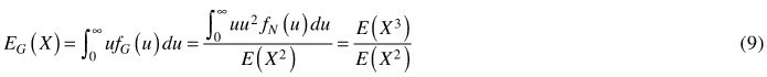
and the mean of the basal-area weighted distribution (Eq. 9) becomes

where the gamma function Γ(k) is a shortcut for the integral ![]() .
.
The cumulative Weibull function has a closed-form expression:
![]()
The closed-form cumulative function makes the computation of quantiles easy. The median (Eq. 11) becomes
![]()
The density of the basal-area weighted diameter distribution (Eq. 3) yields
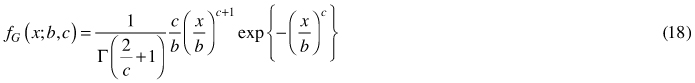
that implies (Gove and Patil 1998) that transformation Y = (x / b)c has the standard gamma distribution with the cumulative distribution function
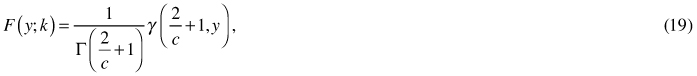
where k = 2 / c + 1 and γ(k), the incomplete gamma function, is a shortcut for the integral ![]() . Although integrals γ(k, y) and Γ(k) cannot be solved in closed forms, they are practically useful because numerical evaluation of the integrals has been implemented in most computing environments. Using the distribution function of Y, the basal-area weighted median diameter (Eq. 12) for the Weibull-distribution of tree diameter can be written as (because the median of a monotonic transformation equals the monotonic transformation of the original median):
. Although integrals γ(k, y) and Γ(k) cannot be solved in closed forms, they are practically useful because numerical evaluation of the integrals has been implemented in most computing environments. Using the distribution function of Y, the basal-area weighted median diameter (Eq. 12) for the Weibull-distribution of tree diameter can be written as (because the median of a monotonic transformation equals the monotonic transformation of the original median):

where F–1(y) is the quantile function of Y that is the inverse function of the standard Gamma cumulative density function.
Finally, Eq. 7 for squared quadratic mean gets form
![]()
2.4 Parameter recovery options
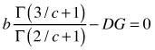
We focused on PRM using the two-parameter Weibull distribution and solving it using the commonly assessed mean or median diameters, such as arithmetic mean (D), basal area-weighted mean (DG), median (DM) and basal area-median (DGM) using the recovery equations (14), (15), (17) and (20), respectively. These equations ensured that the applied mean or median diameter of the stand was equal to the corresponding characteristic computed from the recovered Weibull distribution. In addition, Eq. (21) was used to ensure compatibility with stand density in terms of the number of stems and basal area. The recovery equations are presented in Table 2. As there are two parameters in the Weibull distribution, a recovery needs two of these equations for the system to have a unique solution. Therefore, recovery Methods A–D (See Table 2) were constructed, each of which used the basal area and number of stems and one additional measure for mean or median stand diameter. Note that no matter the mean or median used for solution, the solved two-parameter Weibull function always represents dbh-frequency distribution in this paper. Table 2 lists the equations in the form of finding the roots, f(y) = 0, as they were required in the subroutine funcv for the Newton’s method subroutine newt of the Numerical recipes in FORTRAN (Press et al. 1992, p. 379). The FORTRAN IMSL library was used for solving the parameters (see Appendix).
| Table 2. The recovery equations and their use in Methods A–D. | |
| Recovery equation | Used in Method(s) |
| A | |
 | B |
| C | |
 | D |
| A, B, C, D | |
2.5 Stand characteristics and the height curve
If the stand characteristic required for PRM was not measured in the field, it was predicted. The applied family of models (Siipilehto 2011a) consisted of seemingly unrelated regressions for eight stand characteristics (G, N, D, DGM, H, HGM, DDOM, HDOM) and for the parameters of three optional dbh-distributions along with the height curve. The models were calibrated using linear prediction theory for the best linear unbiased predictor (BLUP) estimation (see Lappi 1991). Known stand characteristics were applied as calibrating variables to improve the expectations for the unknown stand characteristics and unknown parameters of the distribution functions and the height curve. Calibrated (BLUP) estimates for the parameters of Näslund’s (1936) height curve have demonstrated excellent goodness-of-fit (see Siipilehto 2011b, page 28–30). In conclusion, the family of models explored by Siipilehto (2011a) included all the needed sub-models (stand characteristics, dbh distributions, height-dbh relationship) for generating dbh and height for the sample trees of a stand from different combinations of known stand characteristics. In the present study, comparisons between distribution modelling approaches in their capability to generate essential stand characteristics (e.g., assortments volume) were made exactly in the same manner as in Siipilehto (2011a). Although the focus was on Weibull dbh-frequency distribution (WN), the results can be compared similarly with the BLUP estimated basal area-dbh distribution using Weibull (WG) and Johnson’s SB (SBG) functions (Siipilehto 2011a). In addition, a recent SBG model (Siipilehto et al. 2007) and the Weibull height distribution model for young stands (Siipilehto 2009) are compared with the same data in Siipilehto (2011b).
2.6 Validation of the models
Because the BLUP models for stand characteristics included D and DGM, but not DM and DG, only Method A and Method D were validated thoroughly. When predicting the missing stand variable, we started from the assumption that the commonly known stand characteristics, according to guidelines for FMP and for NFI, were available for linear prediction. This presupposed knowledge of the basal area-weighted characteristics (DGM, HGM and G) for advanced stands and arithmetic stand characteristics (D, H and N) for young stands. These variables are referred to later as SOLMU variables (see Solmun maastotyöopas 1997). The most realistic additional characteristics for advanced stands are HDOM and N because they are sometimes additionally required for the aforementioned characteristics (Kuvioittainen arviointi ja... 1998). The combination of known stand characteristics has its effect not only on recovered or predicted dbh-distribution but also on the predicted Näslund’s (1936) height curve. Therefore, both parameters have their effect on generated stand characteristics; recovered or predicted distributions have a particular their effect on generated dbh characteristics: D, DGM and DDOM, in addition to basal area, G, while the predicted height curve has its effect especially on height characteristics, H, HGM and HDOM. Finally, both parameters are needed to derive tree and stand volume. Stand volume and timber assortments were calculated according to models for individual tree volume and a taper curve as a function of known tree dbh and height (Laasasenaho 1982).
The well-known inequality claims that the arithmetic mean, D, is always smaller than the quadratic mean, DQM (Hardy et al. 1988). In practice, it was shown that DGM should be greater than DQM for the unimodal Weibull distribution. When DQM is approaching DGM, the recovered shape parameter c is increasing and the distribution is turning into a peak. We noticed that the BLUP estimated basal area was not accurate enough and sometimes resulted in a DQM that was lower than or equal to D. Note that if this happened, PRM was not able to find the solution. In these cases, we were forced to re-predict basal area. Using the model by Nissinen (2002), the inequality DQM > D was achieved and the parameters could be solved so that the convergence criterion (10–5) was always met.
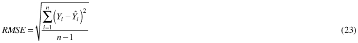
The accuracy of the compared methods was validated in terms of bias (22) and RMSE (23) in the generated stand characteristics, such as stem number, basal area, dominant diameter and height, volume of total growing stock, timber assortments and waste wood fraction. The relative bias and RMSE were calculated by dividing them by the mean value of the observed Yi and they were expressed as percentages.

Using the same data and the same validation criteria as Siipilehto (2011a) and Siipilehto (2011b) means that the results were fully comparable, not only between PPM and PRM methods for the Weibull in this paper but also among all of the models that were previously validated by Siipilehto (2011b). Note that the trees for young stands were sampled from the cumulative Weibull distribution, imitating fixed area sampling, whereas trees for the advanced stands were sampled from the weighted distribution, imitating relascope sampling. A systematic sample of 40 trees was taken from the predicted distributions.
3 Results
3.1 PRM compared with PPM for characterising the variation in N
Method D was used in a 25-year-old Scots pine stand with fixed DGM = 10 cm, G = 10 m2ha–1 and varying stem number, N (ha–1): 3100 for high density, 2500 and 1900 for moderate densities and 1300 for low density forest stands. Comparisons were made between the BLUP estimated (PPM) and recovered (PRM) WN distributions. Similar comparisons between various models can be observed in Siipilehto (2011b, p. 33–34). The BLUP estimation did not respond adequately to the variation in stand density (Fig. 1). Thus, PPM resulted in as high as 27% underestimation in stem number for the highest density and 16% overestimation for the lowest density when the distribution was scaled for the basal area. PRM found converged solutions for these distributions and thus provided correct densities. The resulting variation in the shape of the WN distribution was surprisingly wide. The highest density of 3100 ha–1 resulted in a strongly right-skewed, almost decreasing distribution while the lowest density of 1300 ha–1 resulted in a very peaked distribution and therefore, it was shown with its own Y-axis in Fig. 1. Indeed, in the lowest density, the trees were mostly distributed between the 8 and 11 cm dbh-classes while in the other cases, the trees were distributed between the 1 and 20 cm dbh-classes. In the peaked distribution, DQM (9.896 cm) was close to DGM, resulting in a high value for the shape parameter c (24.5). The only existing PPM that could provide an almost adequate response to the same variation in stem number was the SBG distribution model by Siipilehto et al. (2007), as shown by Siipilehto (2011b, Fig. 5 on p. 34).
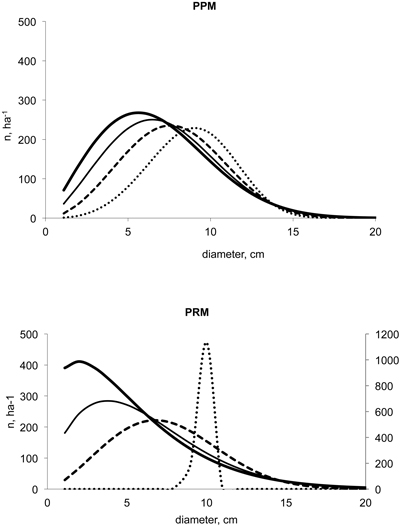
Fig. 1. Two-parameter Weibull distributions predicted with BLUP estimation for PPM (Siipilehto 2011a) and Method D for PRM with respect to variation in N of 3100 (▬), 2500 (─), 1900 (- - -) and 1300 ha–1 (∙∙∙) when DGM was 10 cm and G 10 m2ha–1.
3.2 Localising for a real stand
As in the paper by Siipilehto (2011a), we included the same 21-year-old planted Scots pine stand to study localising the distribution. The observed stand characteristics were as follows: G = 9.6 m2ha–1, N = 949 ha–1, D = 11.0 cm, DGM = 12.4 cm, H = 7.1 m, HGM = 7.5 m, DDOM = 15.7 cm and HDOM = 7.7 m. The PRM (Method A) was used for WN together with BLUP estimation for the unknown stand characteristics. Fig. 2 gives us the observed and the expected W(0) distribution without localisation, in addition to the distributions localised with N, D and H (i.e., W(N, D, H)) and with the varying additional stand characteristics (e.g., W(+G) with the additional basal area). The resulting distributions resembled those in Siipilehto (2011a, Fig. 4). However, the primary difference is the fact that basal area was the most useful additional variable for PRM while it did not calibrate the BLUP estimate for WN effectively (Siipilehto 2011a). The error (overestimation) in total volume with the additional G was 5.3 m3ha–1 (12%) using PPM and only 0.9 m3ha –1 (2%) using PRM. An even smaller error was found using PRM with the additional DGM, namely 0.7 m3ha –1. However, when using the common SOLMU variables (N, D and H), the resulting error was approximately the same, 5 m3ha –1, an overestimation with both PPM and PRM.
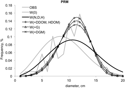
Fig. 2. Parameter recovery method for the 2-parameter Weibull function localised to a real stand. BLUP estimation (Siipilehto 2011a) was used for calibrating the prediction of basal area, if it was unknown.
It is worth mentioning that if parameters were recovered using Method B, C or D (not shown) from the known N and G, together with either DG (12.3 cm), DM (11.1 cm) or DGM, the solution for the parameters were so close to that of Method A that the differences were hardly visible. Indeed, parameter b was always the same 12.06 and c was given values of 4.421, 4.474, 4.458 and 4.466, respectively.
3.3 PRM compared with PPM for generated stand characteristics
Method A for PRM was used in young stands except with the knowledge of N, DGM, HGM and G, when Method D was used instead. The first bars in the Figs. 3–5 represent knowledge of the common SOLMU variables. When the SOLMU variables were assumed to be known in young stands, the RMSE of each validated characteristic was higher in PRM compared with any PPM in the studies by Siipilehto (2011a, b). Included additional HDOM and especially DDOM improved the accuracy in all validated stand characteristics. The knowledge of G in addition to N means that DQM and thus the 2nd raw moment could be derived correctly. This was shown to be a huge improvement in the accuracy of the stand characteristics (Fig. 3). For example, RMSE in total volume was 27% when predicted with SOLMU variables, and the additional dominant tree characteristics reduced RMSE to 22–19%, whereas the additional G provided an RMSE of only 3.5% using Method A and 3.6% using Method D (Fig. 3).
The two rightmost bars in Figs. 3–5 demonstrate that the RMSEs of the validated characteristics were quite comparable, regardless if Method A with D or Method D with DGM was applied in PRM, when both N and G were also known. This comparability was also true in both young and advanced stands. However, in young stands, pulpwood volume as well as HDOM benefited more from DGM knowledge, while waste wood and DDOM were slightly more accurate with a known D. Respectively, in advanced stands, the total volume and HDOM were more accurate with DGM, whereas the volume fractions and DDOM were slightly more accurate with D (Figs. 4 and 5). Finally, knowledge of G and N resulted in an RMSE of only 1.6% in total volume with known DGM while it was 2.8% with D. When N was unknown, the BLUP outcome estimation presented only modest accuracy (RMSE of 20%).
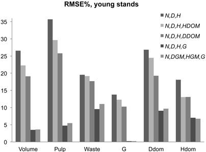
Fig. 3. RMSE% in young stand characteristics using parameter recovery with the BLUP estimation for missing stand variables (Siipilehto 2011a). Method A was used except when G, DGM, HGM and N were known, in which case, Method D was applied.
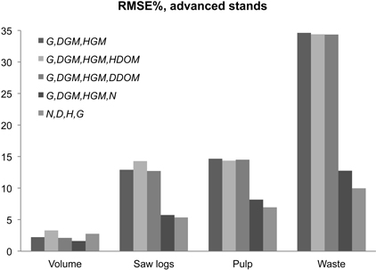
Fig. 4. RMSE% in volume characteristics using parameter recovery with BLUP estimation for missing stand variable in advanced stands (Siipilehto 2011a). Method D was used except when G, D, H and N were known, in which case, Method A was applied.
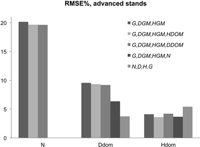
Fig. 5. RMSE% in stem number and dominant tree characteristics using parameter recovery with BLUP estimation for missing stand variables in advanced stands (Siipilehto 2011a).
The compared methods produced different type of biases. In young stands, Siipilehto (2011a) found 4.6% underestimation in total volume with WN, when SOLMU input variables were used as a calibrating variables (Table 3). However, using PRM with the BLUP estimate for basal area, the corresponding bias reached a 12% underestimation. In addition, the same 12% underestimation was also found for DDOM, as was a 9% underestimation of HDOM. The BLUP estimation for WN resulted in the smallest biases in most cases, if the sum characteristics G and N were not also known (Table 3). In general, PRM was superior in terms of bias if both G and N were also known. The residual errors in such a case are given in Fig. 6 for the total volume in young stands using PPM and PRM.
| Table 3. The bias (%) in stand characteristics using the Weibull dbh-frequency distribution for young stands (H < 9 m) with varying combination of known stand characteristics used as calibrating variables. The models included the BLUP estimation for the Weibull by Siipilehto (2011a) and PRM for the Weibull along with the BLUP estimates for the unknown stand characteristics by Siipilehto 2011a. The best validating criteria with respect to the combination of input variables are highlighted in bold. | |||||||
| Model | Predictors | Volume | Pulp | Waste | G | DDOM | HDOM |
| BLUP | N, D, H | 4.6 | 5.7 | 0.3 | 1.4 | 3.5 | 3.6 |
| N, D, H, HDOM | 1.2 | 1.6 | –0.3 | –0.2 | 1.3 | 1.7 | |
| N, D, H,DDOM | 1.7 | 2.3 | –0.8 | –0.1 | 1.3 | 2.6 | |
| N, D, H, G | 2.4 | 2.8 | 0.7 | 0.2 | 1.9 | 2.8 | |
| N, DGM, HGM, G | 1.6 | 2.3 | –1.2 | 0.1 | 1.4 | 2.2 | |
| PRM | N, D, H | 12.3 | 16.0 | –0.9 | 6.6 | 12.4 | 8.5 |
| N, D, H, HDOM | 9.5 | 12.2 | –0.8 | 5.3 | 8.8 | 5.3 | |
| N, D, H,DDOM | 8.1 | 10.5 | –1.1 | 4.4 | 7.3 | 6.1 | |
| N, D, H, G | 0.6 | 0.4 | 1.3 | 0.0 | –2.7 | 1.0 | |
| N, DGM, HGM, G | 0.5 | 0.4 | 1.0 | 0.0 | –2.2 | 1.6 | |
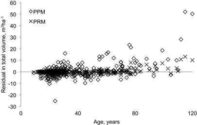
Fig. 6. Residual errors in total volume using BLUP estimation (Siipilehto 2011a) as a parameter prediction model (PPM) or parameter recovery method (PRM) for predicting the Weibull distribution with D, H, N and G as the known stand variables in young stands.
If we compare the WN distribution in advanced stands, PRM resulted in generally lower bias in total and commercial wood volumes but also a higher bias in waste wood volume as well as in stem number and dominant tree characteristics (Table 4). The overestimations of 7% of DDOM and 13–14% of N were the obvious reasons for the 23–24% overestimation in waste wood volume. Indeed, if N and G were known, they were unbiased and the bias in DDOM was reduced to 0.3–1% using PRM. Thus, the determination of the correct DQM through the knowledge of G and N proved essential for the accuracy of PRM. However, no matter the compared method or combination of known stand characteristics, the total volume was always only slightly biased (Table 4) (see also Siipilehto 2011a, b). The approximately 7–10% bias in log and pulpwood volumes using BLUP estimation for WN was reduced to 0–6% using PRM. The best-performing WG distribution in the study by Siipilehto (2011a) also most frequently presented (17 times out of 35 cases) the least biased stand characteristics in the present study. According to the data reported in Table 4, choosing the size distribution model such that the available data and the PPM applied are based on the same scale (i.e., arithmetic stand variables for frequency distribution, weighted medians for basal-area dbh distribution) appears to be essential. In the case of PRM, the mean characteristic used was of no practical importance (Table 4).
| Table 4. The bias (%) in stand characteristics using the Weibull as a dbh-frequency (WN) or basal area-dbh distribution (WG) for advanced stands (H ≥ 9 m) with varying combinations of known stand characteristics used as calibrating variables. The models included the BLUP estimation for the Weibull distribution (Siipilehto 2011a) and PRM for the Weibull function along with the BLUP estimates for the unknown stand characteristics by Siipilehto 2011a. The best validating criteria with respect to the combination of input variables are highlighted in bold. | ||||||||
| Model | Predictors | Volume | Logs | Pulp | Waste | N | DDOM | HDOM |
| WN BLUP | G, DGM, HGM | 1.2 | 10.0 | –9.9 | 1.8 | –1.5 | 1.6 | 0.4 |
| G, DGM, HGM, HDOM | 1.1 | 10.0 | –10.1 | 2.5 | –1.2 | 1.8 | 0.5 | |
| G, DGM, HGM, DDOM | 1.0 | 9.6 | –9.8 | 2.9 | –0.9 | 1.7 | 0.4 | |
| G, DGM, HGM, N | 0.9 | 7.3 | –7.4 | –0.6 | –1.9 | 0.8 | 0.2 | |
| G, D, H, N | –0.9 | 0.2 | –2.7 | 2.0 | 1.7 | –2.8 | –2.3 | |
| WG BLUP | G, DGM, HGM | 0.2 | 1.6 | –2.2 | 5.0 | 2.4 | 0.1 | –0.2 |
| G, DGM, HGM, HDOM | 0.2 | 1.8 | –2.6 | 5.5 | 2.4 | 0.3 | –0.0 | |
| G, DGM, HGM, DDOM | 0.2 | 2.0 | –2.6 | 2.5 | 0.5 | 0.2 | –0.2 | |
| G, DGM, HGM, N | 0.2 | 1.6 | –2.2 | 3.4 | 1.6 | –0.2 | –0.2 | |
| G, D, H, N | –2.3 | –8.7 | 7.8 | 17.2 | 12.4 | –4.7 | –3.0 | |
| WN PRM | G, DGM, HGM | 1.1 | 5.1 | –2.3 | –23.4 | –13.8 | –7.4 | –2.1 |
| G, DGM, HGM, HDOM | 1.8 | 6.4 | –2.2 | –23.3 | –13.0 | –7.2 | –0.3 | |
| G, DGM, HGM, DDOM | 0.7 | 5.1 | –2.9 | –23.9 | –13.5 | –7.3 | –2.1 | |
| G, DGM, HGM, N | –0.1 | 0.8 | –1.6 | 2.8 | 0.0 | –0.3 | –0.5 | |
| G, D, H, N | –0.9 | 0.0 | –2.5 | 1.2 | 0.0 | –1.0 | –1.8 | |
4 Discussion
It is convenient to present various options for parameter recovery in one paper. In addition to the standard moment-based parameter recovery with the arithmetic mean (D) together with the second raw moment, squared quadratic mean dbh, DQM2 (e.g., Lindsay et al. 1996; Cao 2003), we presented equations utilising basal area-weighted mean (DG), median (DM) or basal area-weighted median (DGM) for the recovery of the two-parameter Weibull function. DQM was calculated from either the known or predicted stem number (N) and basal area (G). The Newton-Raphson method for root-finding was used to solve the parameters of the system of two non-linear equations. Because this method appeared somewhat sensitive to the initial guess, we emphasised finding functions for the appropriate initial values of the shape parameter c. The final functions eliminated approximately 50–70% of the needed iterations compared with the use of constant initial values that converged for each stand (see Appendix).
Studies by Siipilehto (2011a; b) in Finland previously indicated that dbh-frequency distribution was superior in young stands, but the weighted, basal area-dbh distribution was a better option in advanced stands in terms of the accuracy in stand characteristics generated from predicted distributions. Similar results have been shown by Gobakken and Næsset (2004) and Palahi et al. (2007). Furthermore, Siipilehto (2011b, p. 33–34) noticed that stem number was not an efficient variable for calibrating the shape of the Weibull distribution, but instead, it was more useful for calibrating the SBG distribution using BLUP estimation. Thus, considerably high RMSE was found in the generated stand density with the Weibull distribution using PPM.
Recently, a great amount of effort has been expended toward calibrating the predicted distribution to achieve compatibility between various input stand characteristics. This has been performed mostly to improve the accuracy in stem volume and assortments (see Kangas and Maltamo 2000a; Kangas and Maltamo 2002; Mabvirura et al. 2002). Note that the calibration estimation presented by Deville and Särndal (1992) necessitates abandoning the smooth shape of the original distribution function. Thus, calibration functions enable mimicking of the irregularities (e.g., bi- or multimodality) of the observed distributions (see Kangas and Maltamo 2000a; Kangas and Maltamo 2003). The Mehtätalo (2004) method, on the other hand, performs the calibration through adjusting directly the predicted diameter percentiles. In contrast, PRM provides a unique solution, keeping the original smooth shape of the unimodal distribution function together with the demonstrated compatibility and without a priori estimated prediction models. In this approach, the irregularities of the observed distribution are more or less brushed aside and regarded as random variation due to sampling. The interesting question raised when applying PRM is how much the achieved compatibility can improve e.g. volume characteristics compared with PPM.
In young stands, PRM was able to yield a clearly lower RMSE for total volume (3.6%) than PPM at its best (8.4% according to Siipilehto 2011a). Conversely, the lowest RMSE for DDOM (3.8%) and HDOM (4.4%) were found using the BLUP estimation for WN as the best option for existing PPMs (Siipilehto 2011a). There are two main reasons for the above results. On one hand, the BLUP estimations for the Weibull distributions (WG and especially for WN) were effectively calibrated with dominant tree characteristics (Siipilehto 2011a) while the applied PRM did not utilise knowledge of dominant tree characteristics, when solving the parameters of the Weibull distribution. Thus, the more accurate DDOM using the BLUP estimated Weibull distribution resulted in the more accurate HDOM as well. On the other hand, the compatibility in the sum characteristics G and N using PRM resulted in a meaningful improvement in volume characteristics. Of the compared PPMs in advanced stands, the BLUP estimation for WG provided the lowest RMSE of 1.7, 5.3 and 7.0% for total, log and pulp wood volumes, respectively, but WN provided the lowest RMSE for waste wood of 11.6% (Siipilehto 2011a). Apart from total volume, the above best results required a large amount of information in addition to common SOLMU variables (see Siipilehto 2011a, Table 10). PRM proved competitive with PPM as long as G and N were both known. For example in volume fractions, PRM provided an RMSE of 5–7% in log and pulp wood volumes, which were quite similar to the best options using PPM. Indeed, the BLUP model for the WG and SBG distribution by Siipilehto et al. (2007) provided an RMSE of 6–8%. Simultaneously, an RMSE in waste wood of 10–13% using PRM was equal to PPMs at their best but clearly lower than PPMs in general (22–25%), when N was a known input variable in addition to SOLMU variables (see Siipilehto 2011b, Fig. 7).
Overall, the results of the PRM were closely related to the accuracy of the models, which were used for the unknown stand characteristics. In this study, the stand characteristics were predicted using BLUP estimation, which enabled calibration of the expectations with the arbitrary set of known stand characteristics under linear prediction theory (see Lappi 1991; Siipilehto 2011a). For PRM, the predictions for G in young stands and predictions for N in advanced stands proved crucial. Burk and Newberry (1984) warned that PRM is very sensitive to small changes in the moment predictions. Because the BLUP estimated basal area was not accurate enough, the solved DQM was sometimes lower than D and PRM was not able to find the solution. For example, with the SOLMU input variables, this outcome was observed 30 times out of 248 cases in young stands. When the Nissinen model (2002) was used for re-predicting basal area, the required inequality D < DQM was achieved. On the other hand, the BLUP estimated N, calibrated with SOLMU variables for advanced stands (i.e., G, DGM and HGM) was suitable for recovery because the resulting DQM was lower than DGM. However, the accuracy in N was unsatisfactory, having an RMSE of 20% and a bias of 13%.
The evaluation data of this study included error-free measurements of the stand characteristics used. In practice, however, the measurements always include errors. Therefore, in a practical situation, the incompatibility of the stand characteristics may lead to lack of solution more often than we observed in this study. Furthermore, the accuracy of the recovered diameter distribution may be lower than demonstrated here with error-free data. Indeed, in Finland, the RMSE in N and G in forest inventory data have varied between 18–81% and 10–32%, respectively. Today, ALS is used in practical forest inventory and ALS based applications have shown similar (Maltamo et al. 2004; Uuttera et al. 2006) or improved accuracy (Suvanto et al 2005; Uuttera et al. 2006; Peuhkurinen et al. 2011; Næsset (2002) compared with the conventional visual assessment of the stand characteristics or photo-interpretation (Kangas et al 2004; Uuttera et al. 2006).
In conclusion, in simulation systems, such as MELA or MOTTI, a considerable number of different types of models are linked together (see Hynynen et al. 2002). Especially in young stands, we are attempting to follow the development of numerous stand characteristics over time in the current version of MOTTI (Siipilehto 2006b). When reaching a threshold of HDOM of 8 m, the followed stand characteristics are converted into individual trees using alternative size distribution models. It is obvious that the sampled trees describing the stand should represent at least those stand characteristics that were used for predicting the distributions. The current PPM models in MOTTI, namely, the Weibull height distribution (Siipilehto 2009) and SBG diameter distribution (Siipilehto et al. 2007), perform quite satisfactorily, but they do not provide compatibility. Strict compatibility, if required, may be difficult to achieve and the solution would require extra calibration functions, such as those shown by Kangas and Maltamo (2000a) and Palahi et al. (2006). However, the compatibility between the three essential stand characteristics is obviously one of the desired features that the presented parameter recovery method can offer. At its best, the parameter recovery method provided superior accuracy for young stands and at least competitive accuracy for advanced stands compared with any existing distribution model used in Finland. In addition, the common belief that the random variable needs weighting for advanced stands proved somewhat controversial. As a whole, the PRM approach can be best improved by improving the accuracy of the forest inventory methods (e.g. Peuhkurinen et al. 2011) and models for the most appropriate stand characteristics. To this end, multivariate multiresponse modelling (see Miina and Saksa 2006; Miina and Heinonen 2008) for stand characteristics are under study. To be able to find a solution for the unimodal Weibull distribution using PRM, we must ensure that the inequalities D < DQM < DGM hold for the input variables in the system of equations, regardless whether they are given as predicted characteristics or determined by measurement or visual assessment.
References
Bailey R.L., Dell T.R. (1973). Quantifying diameter distributions with the Weibull function. Forest Science 19(2): 97–104.
Baldwin V.C. Jr., Feduccia D.P. (1987). Loblolly pine growth and yield prediction for managed West Gulf plantations. USDA Forest Service, Research Paper SO-236. 27 p.
Burk T.J., Newberry J.D. (1984). A simple algorithm for moment-based recovery of Weibull distribution parameters. Forest Science 30(2): 329–332.
Cajanus W. (1914). Über die Entwicklung gleichaltriger Waldbestände: Eine statistische Studie. Acta Forestalia Fennica 3. 142 p.
Cao Q.V. (2004). Predicting parameters of a Weibull function for modelling diameter distribution. Forest Science 50(5): 682–685.
Deville J.C., Särndal C.E. (1992). Calibration estimators in survey sampling. Journal of the American Statistical Association 87: 376–382. http://dx.doi.org/10.2307/2290268.
Dubey S.D. (1967). Some percentile estimators for Weibull parameters. Technometrics 9: 119–129.
Gobakken T, Næsset E. (2004). Estimation of diameter and basal area distributions in coniferous forest by means of airborne laser scanner data. Scandinavian Journal of Forest Research 19: 529–542. http://dx.doi.org/10.1080/02827580410019454.
Gove J.H., Patil G.P. (1998). Modeling the basal area-size distribution of forest stand: a compatible approach. Forest Science 44(2):285–297.
Gustavsen H.G., Roiko-Jokela P., Varmola M. (1988). Kivennäismaiden talousmetsien pysyvät (INKA ja TINKA) kokeet. Suunnitelmat, mittausmenetelmät ja aineistojen rakenteet. Metsäntutkimuslaitoksen tiedonantoja 292. 212 p. [In Finnish].
Haara A., Maltamo M., Tokola T. (1997). The k-nearest-neighbour method for estimating basal-area diameter distribution. Scandinavian Journal of Forest Research 12: 200–208. http://dx.doi.org/10.1080/02827589709355401.
Hardy G.H., Littlewood J.E., Pólya G. (1988). Inequalities. Third edition. Cambridge University Press. 340 p. ISBN 0-521-35880-9.
Holte A. (1993). Diameter distribution functions for even-aged (Picea abies) stands. Meddelelser fra Skogforsk 46(1): 1–47.
Hyink D.M., Moser J.W. (1983). A generalized framework for projecting forest yield and stand structure using diameter distributions. Forest Science 29: 85–95.
Hynynen J., Ojansuu R., Hökkä H., Siipilehto J., Salminen H., Haapala P. (2002). Models for predicting stand development in MELA system. Finnish Forest Research Institute, Research Papers 835. 116 s.
Ilvessalo Y. (1920). Tutkimuksia metsätyyppien taksatoorisesta merkityksestä, nojautuen etupäässä kotimaiseen kasvutaulujen laatimistyöhön. Referat: Untersuchungen über die taxatorische Bedeutung der Waldtypen, hauptsächlich auf den Arbeiten für die Aufstellung der neuen Ertragstafeln Finnlands fussend. Acta Forestalia Fennica 6. 157 p.
Kangas A., Maltamo M. (2000a). Calibrating predicted diameter distribution with additional information. Forest Science 46(3): 390–396.
Kangas A., Maltamo M. (2000b). Percentile based basal area diameter distribution models for Scots pine, Norway spruce and birch species. Silva Fennica 34(4): 371–380.
Kangas A., Maltamo M. (2000c). Performance of percentile based diameter distribution prediction and Weibull method in independent data sets. Silva Fennica 34(4): 381–398.
Kangas A., Maltamo M. (2002). Anticipating the variance of predicted stand volume and timber assortments with respect to stand characteristics and field measurements. Silva Fennica 36(4): 799–811.
Kangas A., Maltamo M. (2003). Calibrating predicted diameter distribution with additional information in growth and yield predictions. Canadian Journal of Forest Research 33(3): 430–434. http://dx.doi.org/10.1139/X02-121.
Kangas A., Heikkinen E., Maltamo M. (2004). Accuracy of partially visually assessed stand characteristics: a case study of Finnish forest inventory by compartments. Canadian Journal of Forest Research 34(4): 916–930. http://dx.doi.org/10.1139/X03-266.
Kilkki P., Päivinen R. (1986). Weibull-function in the esimation of basal area dbh-distribution. Silva Fennica 20(2): 149–156.
Kilkki P., Maltamo M., Mykkänen R., Päivinen R. (1989). Use of the Weibull function in the estimation the basal area dbh-distribution. Silva Fennica 23(4): 311–318.
Knoebel B.R., Burkhart H.E. (1991). A bivariate distribution approach to modeling forest diameter distributions at two points in time. Biometrics 47 : 241–253.
Kuvioittainen arviointi ja tietojen päivitys. (1998). UPM-Kymmene Metsä. 31 p. [In Finnish].
Laasasenaho J. (1982). Taper curve and volume functions for pine, spruce and birch. Communicationes Instituti Forestalis Fenniae 108. 74 p.
Lappi J. (1991). Calibration of height and volume equations with random parameters. Forest Science 37(3): 781−801.
Lappi-Seppälä M. (1930). Untersuchungen über die Entwicklung gleicaltriger Mischbestände aus Kiefer und Birke. Communicationes Instituti Forestalis Fenniae 15(2). 241 p.
Lindsay S.R., Wood G.R., Woollons R.C. (1996). Stand table modelling through the Weibull distribution and usage of skewness information. Forest Ecology and Management 81: 19−23. http://dx.doi.org/10.1016/0378-1127(95)03669-5.
Loetsch F., Zöhrer F., Haller K. (1973). Forest inventory. Vol. II. BLV Verlagsgesellschaft, München. ISBN 3-405-10812-8.
Lönnroth E. (1925). Untersuchungen über die innere Struktur und Entwicklung gleicaltriger naturnormal Kiefernbestände: basiert auf Material aus der Südhälfte Finnlands. Acta Forestalia Fennica 30. 269 p.
Mabvurira D., Maltamo M., Kangas A. (2002). Predicting and calibrating diameter distributions of Eucalyptus grandis (Hill) Maiden plantations in Zimbabwe. New Forests 23: 207–223. http://dx.doi.org/10.1023/A:1020391807554.
Maltamo M. (1997). Comparing basal area diameter distributions estimated by tree species and for the entire growing stock in a mixed stand. Silva Fennica 31(1): 53–65.
Maltamo M., Kangas A. (1998). Methods based on k-nearest neighbour regression in the prediction of basal area diameter distribution. Canadian Journal of Forest Research 28(8): 1107–1115. http://dx.doi.org/10.1139/cjfr-28-8-1107.
Maltamo M., Puumalainen J., Päivinen R. (1995). Comparison of beta and Weibull functions for modelling basal area diameter distribution in stands of Pinus sylvestris and Picea abies. Scandinavian Journal of Forest Research 10: 284–295. http://dx.doi.org/10.1080/02827589509382895.
Maltamo M., Kangas A., Uuttera J., Torniainen T., Saramäki J. (2000). Comparison of percentile based prediction method and the Weibull distribution in describing the diameter distribution of heterogeneous Scots pine stands. Forest Ecology and Management 133: 263–274. http://dx.doi.org/10.1016/S0378-1127(99)00239-X.
Maltamo M., Haara A., Hirvelä H., Kangas A., Lempinen R., Malinen J., Nalli A., Nuutinen T.,, Siipilehto J. (2002a). Läpimittajakaumamalleihin perustuvat vaihtoehdot kuvauspuiden muodostamiseen puuston keskitunnustietojen avulla. Metsätieteen aikakauskirja 3/2002: 407–423. [In Finnish].
Maltamo M., Haara A., Hirvelä H., Kangas A., Lempinen R., Malinen J., Nalli A., Nuutinen T., Siipilehto J. (2002b). MELA2002 ja kuvauspuiden muodostamisen vaihtoehdot. In (Nuutinen, Kiiskinen (eds.) MELA2002 ja käyttöpuun kuvaus. MELA-käyttäjäpäivä 7.5.2002 Joensuu. Metsäntutkimuslaitoksen tiedonatoja 865: 11–31. [In Finnish].
Maltamo M., Eerikäinen K., Pitkänen J., Hyyppä J., Vehmas M. (2004). Estimation of timber volume and stem density based on scanning laser altimetry and expected tree size distribution functions. Remote Sensing of Environment 90: 319–330. http://dx.doi.org/10.1016/j.rse.2004.01.006.
Maltamo M., Suvanto A., Packalén P. (2007). Comparison of basal area and stem frequency diameter distribution modelling using airborne laser scanner data and calibration estimation. Forest Ecology and Management 247: 26–34. http://dx.doi.org/10.1016/j.foreco.2007.04.031.
Mehtätalo L. (2004). An algorithm for ensuring compatibility between estimated percentiles of diameter distribution and measured stand variables. Forest Science 50(1): 20–32.
Mehtätalo L., Maltamo M, Packalén P. (2007). Recovering plot-specific diameter distribution and height-diameter curve using ALS based stand characteristics. International archives of photogrammetry, remote sensing and spatial information sciences 36(3/W52): 288–293. Proceedings of the ISPRS Workshop ‘Laser Scanning 2007 and SilviLaser 2007’ Espoo, September 12–14, 2007, Finland. http://www.isprs.org/proceedings/XXXVI/3-W52/final_papers/Mehtatalo_2007.pdf. [Cited Jan 2013].
Miina J., Saksa T. (2006). Predicting regeneration establishment in Norway spruce plantations using a multivariate multilevel model. New Forests 32: 265–283. http://dx.doi.org/10.1007/s11056-006-9002-y.
Miina J., Heinonen J. (2008). Stochastic simulation of forest regeneration establishment using a multilevel multivariate model. Forest Science 54(2): 206–219.
Mønness E.N. (1982). Diameter distributionds and height curves in even-aged stands of Pinus sylvestris L. Meddelelser fra Norsk Institutt for Skogforskning 36(15): 1–43.
Næsset E. (2002). Predicting forest stand characteristics with airborne scanning laser using a practical two-stage procedure and field data. Remote Sensing of Environment 80: 88–99.
Näslund M. (1936). Skogsförsöksanstaltens gallringsförsök i tallskog. Meddelanden från Statens Skogsförsöksanstalt 29. 169 p. [In Swedish].
Newberry J.D., Burk T.E. (1985). An integrated approach to individual tree volume distribution and stem profile modeling. Canadian Journal of Forest Research 15: 555–560.
Nissinen J. (2002). Improving compatibility between prediction of basal area diameter distributions and assessments of young stands. Metsäsuunnittelun ja -ekonomian pro gradu. University of Joensuu. 48 p.
Packalén P., Maltamo M. (2007). The k-MSN method for the prediction of species-specific stand attributes using airborne laser scanning and aerial photographs. Remote sensing of Environment 109(3): 328–341. http://dx.doi.org/10.1016/j.rse.2007.01.005.
Päivinen R. (1980). On the estimation of stem diameter distribution and stand charactaristics. Folia Forestalia 442: 1–28. [In Finnish with English summary].
Palahi M., Pukkala T., Trasobares A. (2006). Calibrating predicted tree diameter distributions in Catalonia, Spain. Silva Fennica 40(3): 487–500.
Palahi M., Pukkala T. Blasco E., Trasobares A. (2007). Comparison of beta, Johnson’s SB, Weibull and truncated Weibull functions for modelling the diameter distribution of forest stands in Catalonia (north-east of Spain). European Journal of Forest Research 126: 563–571. http://dx.doi.org/10.1007/s10342-007-0177-3.
Peuhkurinen J., Maltamo M., Malinen J. (2008). Estimating species-specific diameter distributions and saw log recoveries of boreal forests from airborne laser scanning data and aerial photographs: a distribution-based approach. Silva Fennica 42(4): 625–641.
Peuhkurinen J., Mehtätalo L., Maltamo M. (2011). Comparing individual tree detection and the area-based statistical approach for retrieval of forest stand characteristics using airborne laser scanning in Scots pine stands. Canadian Journal of Forest Research 41: 583–598. http://dx.doi.org/10.1139/X10-223.
Poudel K.P. (2011). Evaluation of methods to predict Weibull parameters for charcterizing diameter distributions. Electronic Thesis & Dissertation Collection. Lousiana State University. http://etd.lsu.edu/docs/available/etd-06302011-133644/unrestricted/Poudel_Thesis.pdf. [Cited Jan 2013].
Press W.H., Teukolsky S.A., Vetterling W.T., Flannery B.P. (1992). Numerical recipes in FORTRAN: the art of scientific. 2nd ed. Cambridge University Press. 963 p.
Ruuska J., Siipilehto J., Valkonen S. (2008). Effect of edge stand on the development of young Pinus sylvestris stands in southern Finland. Scandinavian Journal of Forest Research 23: 214−226. http://dx.doi.org/10.1080/02827580802098127.
Sarkkola S., Alenius V., Hökkä H., Laiho R., Penttilä T., Päivänen J. (2003). Changes in structural inequality in Norway spruce stands after water-level drawdown. Canadian Journal of Forest Research 33: 222–231. http://dx.doi.org/10.1139/X02-179.
Sarkkola S., Hökkä H., Laiho R., Päivänen J., Penttilä T. (2005). Stand structural dynamics on drained peatlands dominated by Scots pine. Forest Ecology and Management 206: 135–152. http://dx.doi.org/10.1016/j.foreco.2004.10.064.
Shiver B.D. (1988). Sample sizes and estimation methods for the Weibull distribution for unthinned slash pine plantation diameter distributions. Forest Science 34(3): 809–814.
Siipilehto J. (1999). Improving the accuracy of predicted basal-area diameter distribution in advanced stands by determining stem number. Silva Fennica 33(4): 281–301.
Siipilehto J. (2006a). Height distributions of Scots pine sapling stands affected by retained tree and edge stand competition. Silva Fennica 40(3): 473–486.
Siipilehto J. (2006b). Linear prediction application for modelling the relationships between a large number of stand characteristics of Norway spruce stands. Silva Fennica 40(3): 517–530.
Siipilehto J. (2009). Modelling stand structure in young Scots pine dominated stands. Forest Ecology and Management 257: 223–232. http://dx.doi.org/10.1016/j.foreco.2008.09.001.
Siipilehto J. (2011a). Local prediction of stand structure using linear prediction theory in Scots pine-dominated stands in Finland. Silva Fennica 45(4): 669–692.
Siipilehto J. (2011b). Methods and applications for improving parameter prediction models for stand structures in Finland. Dissertationes Forestales 124. 56 p. http://www.metla.fi/dissertationes/df124.htm. [Cited Jan 2013].
Siipilehto J., Heikkilä R. (2005). The effect of moose browsing on the height structure of Scots pine saplings in a mixed stand. Forest Ecology and Management 205: 117–126. http://dx.doi.org/10.1016/j.foreco.2004.10.051.
Siipilehto J. Sarkkola S., Mehtätalo L. (2007). Comparing regression estimation techniques when predicting diameter distributions of Scots pine on drained peatlands. Silva Fennica 41(1): 333–349.
Solmun maastotyöopas. (1997). Metsätalouden kehittämiskeskus Tapio. 82 s. [In Finnish].
Tham Å. (1988). Structure of mixed Picea abies (L.) Karst. and Betula pendula Roth and Betula pubescens Ehrh. stands in South and Middle Sweden. Scandinavian Journal of Forest Research 3: 355–369.
Uuttera, J, Anttila P., Suvanto A., Maltamo M. (2006). Yksityismetsien metsävaratiedon keruuseen soveltuvilla kaukokartoitusmenetelmillä estimoitujen puustotunnusten luotettavuus. Metsätieteen aikakauskirja 4/2006: 507–519. [In Finnish].
Valkonen S. (1997). Viljelykuusikon alkukehityksen malli. Metsätieteen aikakauskirja 3/1997: 321–347. [In Finnish].
Valkonen S., Ruuska J., Siipilehto J. (2002). Effect of retained trees on the development of young Scots pine stands in Southern Finland. Forest Ecology and Management 166(1–3): 227–243.
Vetterling W.T., Teukolsky S.A., Press W.H., Flannery B.P. (1992). Numerical recipes: example book (FORTRAN). 2nd ed. Cambridge University Press. 245 p.
Total of 76 references
Appendix
The IMSL library functions GAMMA(k) and GAMIN(P,k) and numerical recipes (Press et al. 1992) were used to solve the parameters of the two-parameter Weibull function in FORTRAN. Solving the non-linear systems of equations was achieved by the Newton-Raphson root-finding algorithm using the subroutine newt (Vetterling et al. 1992, p. 131). This method appeared somewhat sensitive to the initial parameter guesses. The parameter b (represent 63rd percentile) was set to DQM. The initial value c from 2 to 3 could be used as a relevant range for the fixed initial value for the shape parameter. However, utilising the high correlation between c and two differently defined mean characteristics (see Siipilehto 2009) and developing it with a trial and error method, we found satisfied equations for c_ini as follows:
c_ini = 1/ln(DQM4/Da4 + 0.1) and
c_ini = 1/ln(Db 2/ DQM2 + 0.05),
where Da is either D or DM and Db is either DG or DGM, respectively.
Fig. A1 shows that the initial guess was quite accurate until the value of approximately c = 10. The tested constant initial values of c_ini of 2.0 and 3.0 needed a total of 10891–23037 and 7277–11078 iterations when Methods A, B and D were applied. The functions for the initial values reduced the requirement to 5232–5449 iterations. Thus, in the data set consisting of 467 stands, the functions resulted in an average of approximately12 iterations/stand.
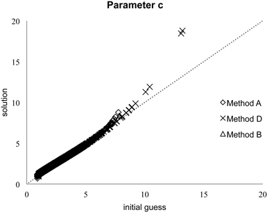
Fig. A1. Initial guess and the final solution for the shape parameter c of the Weibull function.
