Per-Ola Olsson  ,
Tuula Kantola,
Päivi Lyytikäinen-Saarenmaa,
Anna Maria Jönsson,
Lars Eklundh
,
Tuula Kantola,
Päivi Lyytikäinen-Saarenmaa,
Anna Maria Jönsson,
Lars Eklundh
Development of a method for monitoring of insect induced forest defoliation – limitation of MODIS data in Fennoscandian forest landscapes
Olsson P.-O., Kantola T., Lyytikäinen-Saarenmaa P., Jönsson A. M., Eklundh L. (2016). Development of a method for monitoring of insect induced forest defoliation – limitation of MODIS data in Fennoscandian forest landscapes. Silva Fennica vol. 50 no. 2 article id 1495. https://doi.org/10.14214/sf.1495
Highlights
- We developed and tested a method to monitor insect induced defoliation in forests based on coarse-resolution satellite data (MODIS)
- MODIS data may fail to detect defoliation in fragmented landscapes, especially if defoliation history is long. More homogenous forests results in higher detection accuracies
- The method may be applied to future coarse and medium-resolution satellite data with high temporal resolution.
Abstract
We investigated if coarse-resolution satellite data from the MODIS sensor can be used for regional monitoring of insect disturbances in Fennoscandia. A damage detection method based on z-scores of seasonal maximums of the 2-band Enhanced Vegetation Index (EVI2) was developed. Time-series smoothing was applied and Receiver Operating Characteristics graphs were used for optimisation. The method was developed in fragmented and heavily managed forests in eastern Finland dominated by Scots pine (Pinus sylvestris L.) (pinaceae) and with defoliation of European pine sawfly (Neodiprion sertifer Geoffr.) (Hymenoptera: Diprionidae) and common pine sawfly (Diprion pini L.) (Hymenoptera: Diprionidae). The method was also applied to subalpine mountain birch (Betula pubescens ssp. Czerepanovii N.I. Orlova) forests in northern Sweden, infested by autumnal moth (Epirrita autumnata Borkhausen) and winter moth (Operophtera brumata L.). In Finland, detection accuracies were fairly low with 50% of the damaged stands detected, and a misclassification of healthy stands of 22%. In areas with long outbreak histories the method resulted in extensive misclassification. In northern Sweden accuracies were higher, with 75% of the damage detected and a misclassification of healthy samples of 19%. Our results indicate that MODIS data may fail to detect damage in fragmented forests, particularly when the damage history is long. Therefore, regional studies based on these data may underestimate defoliation. However, the method yielded accurate results in homogeneous forest ecosystems and when long-enough periods without damage could be identified. Furthermore, the method is likely to be useful for insect disturbance detection using future medium-resolution data, e.g. from Sentinel‑2.
Keywords
remote sensing;
insect defoliation detection;
coarse-resolution;
EVI2;
z-score;
Sentinel-2
-
Olsson,
Lund University, Department of Physical Geography and Ecosystem Science, Sölvegatan 12, S-223 62 Lund, Sweden
E-mail
per-ola.olsson@nateko.lu.se
- Kantola, Texas A & M University, Knowledge Engineering Laboratory, Department of Entomology, College Station, TX, USA E-mail tuula.kantola@helsinki.fi
- Lyytikäinen-Saarenmaa, University of Helsinki, Department of Forest Sciences, P.O. Box 27, FI-00014 University of Helsinki, Finland E-mail paivi.lyytikainen-saarenmaa@helsinki.fi
- Jönsson, Lund University, Department of Physical Geography and Ecosystem Science, Sölvegatan 12, S-223 62 Lund, Sweden E-mail anna_maria.jonsson@nateko.lu.se
- Eklundh, Lund University, Department of Physical Geography and Ecosystem Science, Sölvegatan 12, S-223 62 Lund, Sweden E-mail lars.eklundh@nateko.lu.se
Received 13 September 2015 Accepted 18 January 2016 Published 3 February 2016
Views 232790
Available at https://doi.org/10.14214/sf.1495 | Download PDF

1 Introduction
Insect outbreaks can result in altered structure and functioning of forest ecosystems, as well as influence tree species composition and forest succession (Linke et al. 2007; Dix et al. 2009). Severe defoliation by insects can influence carbon dynamics with a reduced uptake of carbon due to reductions of photosynthesis (Kurz et al. 2008; Jepsen et al. 2009; Heliasz et al. 2011), which in turn can lead to reduced growth and economic losses. For example, in Finland the estimated average annual economic loss of a single year of defoliation by the European pine sawfly (Neodiprion sertifer Geoffr.) (Hymenoptera: Diprionidae) can reach up to $40·ha–1, and by the common pine sawfly (Diprion pini L.) (Hymenoptera: Diprionidae) up to $310·ha–1 (Lyytikäinen-Saarenmaa and Tomppo 2002). As a consequence of climate change, insect outbreaks are predicted to become more frequent (Björkman et al. 2011; Netherer and Schopf 2012). Insect populations may experience increased survival, development, reproduction, and dispersal rates due to increasing temperatures (Logan et al. 2003; Lindner et al. 2010). A number of forest insects have already begun to expand their normal ranges of distribution (Vanhanen et al. 2007; Jepsen et al. 2008; Hlásny et al. 2011), or change their status into disturbance agents within their original distributions (De Somviele et al. 2007). Hence, mapping and monitoring of insect outbreaks is a highly important topic that calls for development of cost-efficient technologies, such as satellite based remote sensing applications (Lyytikäinen-Saarenmaa et al. 2008; Kantola et al. 2010).
Remote sensing provides a vast array of efficient tools for forest disturbance detection, including mapping of insect induced defoliation; see reviews in (Wulder et al. 2006; Adelabu et al. 2012; Rullan et al. 2013). Besides the use of aerial photography or data from meter-resolution satellites, which may be unavailable or very expensive, several remote sensing applications for insect damage detection have been developed based on medium spatial resolution (10−30 m) satellite data: Landsat Thematic Mapper (TM) images have been used in mapping damage by the mountain pine beetle (Dendroctonus ponderosae Hopkins) (Franklin et al. 2003; Skakun et al. 2003; Goodwin et al. 2008; Coops et al. 2010), and the common pine sawfly (Ilvesniemi 2009). Système Pour l’Observation de la Terre (SPOT) data have been used to map Hungarian spruce scale (Physokermes inopinatus Danzig and Kozfir) damage (Olsson et al. 2012). Remote sensing data at medium-resolution has been provided for large areas by the opening of the Landsat archive (Wulder et al. 2012), and methods to map different forest disturbance types from this long data record have been successfully developed (Cohen et al. 2010; Kennedy et al. 2010; Meigs et al. 2011; Zhu et al. 2012). Based on Landsat, annual global forest cover change maps have been created (Townshend et al. 2012; Hansen et al. 2013). However, medium spatial resolution sensors have low temporal resolution (e.g. 16 days revisit time for Landsat). This long interval between images is a limitation for insect defoliation monitoring in many areas since many insects only have a short period when an outbreak is detectable (Rullan-Silva et al. 2013), and cloudy conditions may result in a situation with no available medium-resolution images during an outbreak. This precludes the use of some of the otherwise successful general forest disturbance monitoring methods (e.g. Kennedy et al. 2010) for detecting insect defoliation. To reduce the problems with clouds, pixel-wise time-series have been created to detect general forest disturbances (Zhu et al. 2012) and to create phenological profiles (Melaas et al. 2013). However, in Fennoscandia it is not uncommon to have few or even no cloud-free Landsat scenes during an entire growing season. For example, for one of the insect outbreaks included in this study there were only small fractions of the disturbed areas visible in Landsat images during the outbreak. These conditions limits the use of currently available medium-resolution data for insect disturbance monitoring
To achieve daily temporal resolution, the only current data source for large-area monitoring of forest disturbances is low spatial resolution (250−1000 m) satellite data. In general, these data are freely available with global cover. Several low spatial resolution sensor systems have been used in insect disturbance monitoring; for example, data from the National Oceanic and Atmospheric Administration (NOAA) Advanced Very High Resolution Radiometer (AVHRR), the Moderate Resolution Imaging Spectroradiometer (MODIS), and SPOT VEGETATION were utilized by Kharuk et al. (2004, 2007, 2009) to monitor damage by the Siberian silk moth (Dendrolimus superans sibiricus Tschetverikov) in Siberia. MODIS data have also been used to detect defoliation by the European gypsy moth (Lymantria dispar L.) (de Beurs and Townsend 2008; Spruce et al. 2011) in North America, and SPOT VEGETATION and NOAA AVHRR data were used by Fraser et al. (2005) to monitor changes in forest cover at continental scale. The high acquiring frequency (daily) of MODIS has been utilized in several studies to perform time-series analysis to detect insect disturbance: Jepsen et al. (2009) performed a time-series analysis with MODIS Normalized Difference Vegetation Index (NDVI) to monitor outbreaks of the autumnal moth (Epirrita autumnata Borkhausen) and the winter moth (Operophtera brumata L.) in mountain birch (Betula pubescens ssp. Czerepanovii N.I. Orlova) forests in northern Fennoscandia; Eklundh et al. (2009) successfully mapped defoliation by the European pine sawfly in southeastern Norway; and Anees and Aryal (2014) developed methods based on MODIS data for near real-time detection of bark beetle infestations on pine forest in North America. Insect disturbances have also been included as a class in general forest disturbance monitoring methods based on MODIS data (Sulla-Menashe et al. 2014). These studies provide evidence of the general potential of low spatial resolution data with high temporal resolution for mapping of insect defoliation. With a number of new coarse-resolution satellite system being launched (e.g. the American Joint Polar Satellite System (JPSS) Visible Infrared Imaging Radiometer (VIIRS) (JPSS 2015) and the European Sentinel-3 Ocean and Land Color Instrument (OLCI) (ESA 2015b)) the provision of global data with a historical continuity with MODIS is ensured for several years to come. It is important to establish if this type of remote sensing data is useful for general insect damage monitoring in forests.
It can be noted that several of the cited MODIS-based studies have been conducted in large homogenous forest areas, and it is questionable if the spatial resolution of MODIS is sufficient for monitoring also of fragmented and intensively managed forests. The difficulty in these areas is further aggravated by the low spatial precision for the 250 m resolution MODIS data due to gridding artefacts (Tan et al. 2006). Furthermore, the reflectance of a single MODIS pixel is recorded over an area on the ground that may be considerably larger than the nominal size of the pixel, and varying with the viewing angle (Townshend et al. 2000). It is also not clear how generally applicable the developed MODIS based disturbance detection methods are, as many studies are tailored for specific insects and outbreak events. It is therefore likely that mapping accuracies strongly depend on spatial scale, pattern and intensity of an attack, as well as the data used. To investigate the possibility to use data at MODIS spatial resolution for general insect defoliation monitoring in Fennoscandian forests with different levels of fragmentation we selected three study areas with known insect defoliation and with different characters: two managed and fragmented forests in eastern Finland that mostly consist of pure Scots pine (Pinus sylvestris L.) (pinaceae) stands, and with different insect outbreak histories; and one unmanaged deciduous birch forest in northern Sweden of patchy and rather sparse character. Even with the highest available spatial resolution for MODIS (250 m) this inevitably leads to mixed pixels and challenging conditions for detecting defoliation.
Our overall study aim was to analyse the potential to use time-series methodology applied to high temporal resolution remotely sensed data for insect disturbance monitoring in fragmented forest landscapes in Fennoscandia. This will demonstrate the accuracy of regional or global disturbance monitoring methods based on current and future coarse-resolution sensor data in Fennoscandian forest landscapes, and also indicate the potential of future high temporal resolution medium spatial resolution data, e.g. Sentinel-2. Two specific study objectives were defined: (1) to develop and apply a general forest defoliation detection method based on MODIS data, and (2) to test the accuracy and discuss the limitations of these data in different forest landscapes with different defoliators, levels of fragmentation and outbreak histories.
2 Materials and methods
2.1 Study areas
2.1.1 Eastern Finland
The study areas in eastern Finland were selected due to well documented insect outbreaks with available time-series of defoliation data. They are located in the municipalities of Ilomantsi (62°53´N, 30°54´E) and Outokumpu (62°46´N, 28°57´E) (Fig. 1). The growing season is around 160 days, and the annual mean temperature (1950–2013) is 3.3 °C. January and February are the coldest months with mean temperatures of –10.2 °C, and July is the warmest month with a mean temperature of 16.5 °C (data derived from the E-OBS dataset; Haylock et al. 2008). These landscapes are generally flat and mostly covered by managed forests dominated by Scots pine. The main forest site types in both areas are poor and dry heath of Calluna type, quite poor and dryish heath of Vaccinium type, and medium fertile fresh heath of Myrtillus type (Cajander 1926). Landscapes in both areas are fragmented with heavily managed forests; the average size of a forest stand in both study areas is between 1 and 3 ha, which means that MODIS pixels are likely to contain fractions of different forest stands, clear cut areas, water, etc.
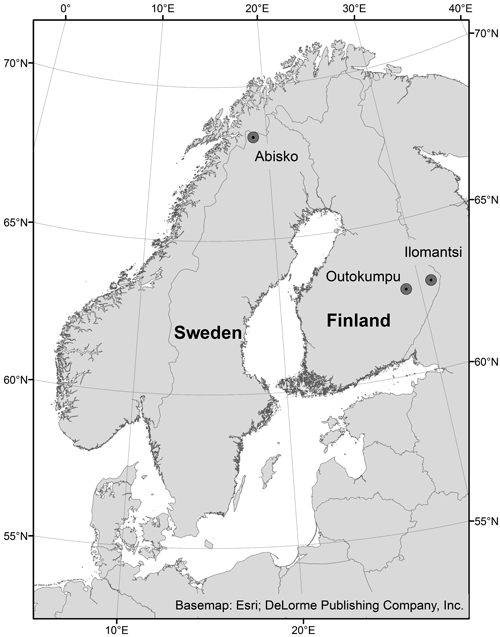
Fig. 1. The two study areas in Outokumpu and Ilomantsi, eastern Finland, and the Abisko study area, northern Sweden. Reference system: WGS84.
Outbreak frequencies, as well as spatial and temporal scales of outbreaks by pine sawflies have experienced changes during the recent decades in Finland (De Somviele et al. 2007; Talvitie et al. 2011). In Ilomantsi, the first symptoms of a common pine sawfly outbreak were visible already in 1999. The outbreak has resulted in notable damage including tree mortality within an area of approximately 10 000–15 000 ha. Ilomantsi was the eastern edge of a 500 000 ha wide outbreak, the largest outbreak in the Finnish forest health records (De Somviele et al. 2007). Until present, population density and defoliation intensity, as well as the spatial extent of the damage have been fluctuating. In Outokumpu, the outbreak history is shorter. A progradation phase of the European pine sawfly populations started in 2008 within an area of approximately 50 000 ha. Population densities reached the peak in 2011 and started to collapse into a postgradation phase.
2.1.2 Northern Sweden
Abisko (68°21´N, 18°48´E) (Fig. 1) is located in the subalpine zone in northern Sweden. The area is mainly covered by unmanaged mountain birch forests, mires and heath vegetation with dwarf shrubs, grasses and lichens (Wielgolaski 2001). Birch forests in the area are infested by the autumnal moth and the winter moth in time intervals of 9−10 years, resulting in severe defoliation (Bylund 1995; Tenow et al. 2007). The latest outbreaks occurred in 2004 (Heliasz et al. 2011) and 2012−2013 (Bengt Landström, County administrative board of Norrbotten, pers. comm. 31.10.2013). These outbreaks may have substantial impact on the birch forests and result in long periods of recovery or mortality (Tenow 1996). The mean annual temperature has been around 0 °C during the last century (Callaghan et al. 2010) with January and February as the coldest months with a mean temperature of –10.7 °C, and July the warmest month with a mean of 11.7 °C. The growing season is around 140 days (monthly means and length of growing season derived from climate data from Abisko Scientific Research Station 2015). Increasing temperatures since 2000 have resulted in mean annual temperatures above 0°C (Callaghan et al. 2010). Warmer temperatures, especially a lower frequency of years with extremely cold winters (Callaghan et al. 2010) strongly influence birch moth populations (Babst et al. 2010). The autumnal moth has a mortality threshold of –36 °C (Tenow and Nilssen, 1990) and the winter moth is slightly more sensitive to low temperatures (Jepsen et al. 2008).
2.2 Data
2.2.1 Defoliation assessment data
Eastern Finland
In Ilomantsi, the first permanent plots for monitoring the common pine sawfly outbreak were established in 2002. In Outokumpu, the first permanent plots for monitoring the European pine sawfly outbreak were established in 2009. When sampling these areas, centers of sampling plots (radius 8−13 m) were located with a Trimble Pro XH GPS devise (Trimble Navigation Ltd., Sunnyvale, CA, USA). Tree-wise defoliation intensity was assessed annually following a method by Eichhorn (1998): The foliage of each individual tree was observed from different directions, and the defoliation level was assessed as the tree specific loss of foliage in comparison with a healthy tree with full foliage, growing on the same site type and canopy cover layer. The plot-wise mean defoliation levels were calculated as the average defoliation of the trees from the two upper canopy cover layers (for further information on defoliation assessment, see Kantola et al. 2010).
In addition to the permanent plots, a defoliation assessment over a larger area was performed at stand level in June 2010. The mean defoliation for each forest stand was visually estimated and classified into two classes: healthy (< 20% of mean defoliation) and defoliated (≥ 20% of mean defoliation). This dataset was used for evaluation and is referred to as the evaluation data. The assessment included 87 Scots pine stands in Ilomantsi; 65 of these stands were healthy and 22 defoliated. In Outokumpu the assessment included 43 stands with 35 damaged and 8 healthy stands.
Northern Sweden
In Abisko, the field sampling was performed with the sole purpose to collect field data of defoliation for this study, and was hence performed with a different method compared to that in Finland. The method was specifically developed to efficiently map the extensive outbreak of autumnal moth in 2013, and the field sampling was performed during the last week of June that year. Since MODIS data were utilized in the study, defoliation assessments were performed over sampling units covering the nominal extent of one MODIS pixel with 250 m spatial resolution. A grid representing the nominal pixels was created and transformed from MODIS sinusoidal projection (LPDAAC 2012d) to the Swedish projection SWEREF99 TM. The sampling units were selected with the aim to obtain a large spatial coverage with even spatial distribution, and were located in the field with the aid of a Pocket LOOX N520 PDA (Fujitsu Siemens Computers, Darmstadt, Germany) with built-in GPS and 1-m spatial resolution orthophotos. For each sampling unit, the level of defoliation was assessed visually. For units with evenly distributed defoliation and high visibility, the assessment was performed along two sides and one diagonal of the MODIS pixel; the sides were chosen so that all four corners of a pixel were visited. For sampling units with unevenly distributed defoliation intensity or poor visibility, the assessment was performed along both diagonals and all sides. Due to the difficulty to assess the defoliation degree with high accuracy over an entire MODIS pixel only two classes were used in this study: (1) pixels with defoliation of at least 50%, and (2) pixels with less than 50% defoliation. A classification into these two categories was generally not difficult to perform since the birch trees were either heavily defoliated or nearly healthy within a majority of the sampling units. The two classes were labelled as “healthy” and “defoliated” since most sampling units with less than 50% of defoliation were only mildly defoliated. A total of 80 sampling units (250 m × 250 m) were assessed, yielding 48 damaged and 32 healthy units.
2.2.2 Satellite data
Two Terra/MODIS satellite sensor data products were utilized in this study: (1) MOD09Q1 (ver. 5), surface reflectance in the red and near infrared (NIR) bands in 8-day periods with 250 m spatial resolution (LPDAAC 2012a) and (2) MOD09A1 (ver. 5), surface reflectance in 8-day periods with 500 m spatial resolution (LPDAAC 2012b); these data were used solely for quality assurance (QA) information. It has been suggested that data from the MODIS sensor on board the Aqua satellite should be preferred to data from the Terra/MODIS sensor due to the sensor degeneration mainly influencing Terra/MODIS (Wang et al. 2012). The sensor drift is however small, mainly influencing detection of subtle trends. Nevertheless, as a cautious approach we plotted time-series of MODIS Terra and MODIS Aqua 16-day NDVI (LPDAAC 2012c) and made a visual comparison, but no obvious difference was indicated. Hence, we did not consider the drift to be a limitation to our study.
2.3 Method development
Four general steps were taken to develop the method to be applied in both study areas: (1) red and near infrared (NIR) reflectances were extracted from the MOD09Q1 data, and vegetation indices were computed; (2) time-series were created from these vegetation indices and processed with the TIMESAT software (Jönsson and Eklundh 2002, 2004) to find a metric to represent the forests health condition for a season; (3) mean and standard deviation during healthy conditions were estimated for this metric; and (4) the MODIS pixels were classified into damaged or healthy based on z-scores of the metric. Details are given below.
2.3.1 Vegetation indices
Due to the level of landscape fragmentation, only MODIS data with the highest spatial resolution (250 m) were used. This precludes the use of other spectral bands than red and NIR. In this study, we tested NDVI, the Enhanced Vegetation Index (EVI), the 2-band Enhanced Vegetation Index (EVI2) and the Wide Dynamic Range Vegetation Index (WDRVI). NDVI (Rouse et al. 1973; Tucker 1979) has been widely used in ecological studies. However, a limitation is that NDVI can reach saturation in high biomass regions, such as forested areas (Huete et al. 1997). Huete et al. (2002) developed EVI, which includes blue, red and NIR wavelength bands, to enhance the signal from vegetation in high biomass regions. Jiang et al. (2008) developed EVI2 as a two-band version of EVI, utilizing red and NIR bands, and showed that there were no significant differences between EVI and EVI2. WDRVI is a similar vegetation index, based on red and NIR spectral bands that also was developed to improve the sensitivity in high biomass regions (Gitelson 2004). WDRVI has been used to detect Scots pine defoliation by insects, with similar results as NDVI (Eklundh et al. 2009). Initial tests between defoliation data and vegetation indices indicated that damage could not be detected with EVI (LPDAAC 2012c) or WDRVI with high accuracy in the study area. Hence, only NDVI and EVI2 were studied further. These indices were computed according to Eqs. 1 and 2.
2.3.2 Time-series creation and TIMESAT processing
Time-series of NDVI and EVI2 with a temporal resolution of eight days were generated for the years 2001−2011 and processed with TIMESAT ver. 3.2. (Jönsson and Eklundh 2002, 2004). In TIMESAT, noise is reduced by fitting smooth functions to time-series of data, and seasonality parameters, such as start and end of a growing season, are extracted. In this study, the seasonality parameter giving the maximum value of the fitted function during a season, from here on called “season max”, was used as a metric for the forest condition of a season (Fig. 2). An advantage of season max compared to methods based on single data points or averages over short periods, is that season max is based on weighted data from the entire growing season; hence, it is relatively insensitive to noise and outliers.
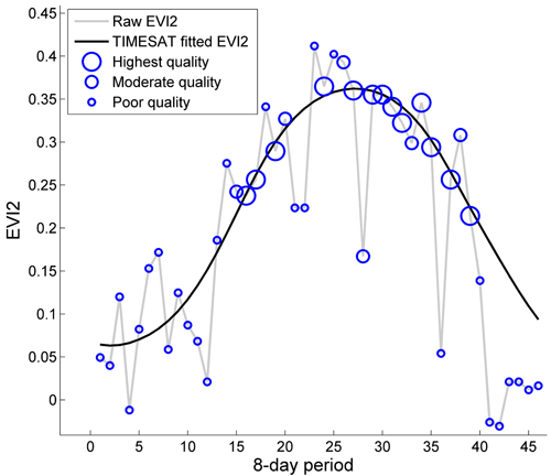
Fig. 2. MODIS derived 2-band Enhanced Vegetation Index (EVI2) (grey line) and EVI2 fitted in TIMESAT with a double logistic function (black line) for the year 2001 and one MODIS pixel in the Outokumpu area. Blue circles show the quality of the data, with large circles for high quality and small circles for low quality. Season max, the seasonality parameter used in this study, is the maximum vegetation index value of the TIMESAT fitted function.
Weights were assigned to each data value in TIMESAT to suppress the influence of data with poor quality on the fitted functions (see Fig. 2, where the size of circles represents the MODIS data quality). Pixels with the highest quality were assigned a weight of 1.0, moderate quality a weight of 0.8, and poor quality a weight of 0.1, where the quality is an overall indicator of data reliability based on quality assurance (QA) flags from both MOD09Q1 and MOD09A1. The reason for including MOD09A1 is that these quality data are more comprehensive, including e.g. solar zenith angle. Pixels were assigned the highest quality only if all QA flags indicated no disturbance and the solar zenith angle was low. The quality was downgraded to moderate if the cloud status was mixed, the solar zenith angle was higher than 82°, or if any of the other QA flags indicated disturbance. Pixels were considered to be of poor quality if disturbance was indicated in the QA flags or the solar zenith angle was higher than 86°. Pixels with no cloud status set, but “assumed clear”, according to Vermote et al. (2011), were downgraded to medium quality.
Potential outliers were removed with the median method available in TIMESAT (Jönsson and Eklundh 2002, 2004), and no adaptation to an upper envelope was performed. All three fitting functions available in TIMESAT ver. 3.2 were tested to derive season max: Savitzky-Golay filtering, asymmetric Gaussian and double logistic functions. Gaussian and logistic functions result in smooth curves and have the advantage of only few parameters to be set. Savitzky-Golay filtering, on the other hand, has the advantage that the fitted function follows the vegetation index data more closely, and hence, might be better for detecting smaller deviations. However, with a larger number of parameters Savitzky-Golay filtering requires more work to be fine-tuned. In areas with different seasonal trajectories the method requires slightly different settings, making the method less general.
2.3.3 Statistical decision criteria
In order to make the method more general and less reliant on absolute thresholds for damage detection we based our analyses on z-scores. A z-score is the number of standard deviations a data value deviates from the mean value of a dataset, thereby taking the natural variability of a pixel into account. Hence, a deviation in a dataset with large variance will result in a lower z-score, compared to the same absolute deviation in a dataset with low variance. Z-scores have proven valuable in similar types of analyses, e.g. drought monitoring (Peters et al. 2002).
The mean and standard deviation of season max had to be estimated for each pixel at healthy conditions (no disturbance) before z-scores were computed. In this study we use the term “reference condition” to represent healthy conditions. The reference condition is unique for each pixel and defined as the mean and standard deviation of season max for years with no or little disturbance. We assumed that high vegetation index values represent healthy conditions. Hence, the reference condition for a pixel is computed as follows: (1) identify the n years with highest season max, where n is the number of years that gives the highest detection accuracy; and (2) estimate mean and standard deviation for season max based on these n years.
We began the method development with the data from Finland. Although the Ilomantsi area had the longest time-series of defoliation assessment available, a difficulty was that the duration of the insect outbreak was as long as the entire time-series of MODIS data. In addition, the outbreak has led to forestry activities, such as salvage cutting, around some defoliation assessment plots. Hence, the number of years without disturbance in Ilomantsi to identify reference conditions was insufficient. For this reason only plots from Outokumpu were included in the method development.
Since the spatial precision of the 250 m MODIS data is low (Tan et al. 2006), only training plots located in stands covering nearly entire MODIS pixels were included in the method development; this resulted in a total of 10 plots. Each mean defoliation estimate was considered as an independent observation regardless of year of assessment, i.e. each plot contributed with 3 values, one for each of the years with defoliation assessment 2009−2011, resulting in a total of 30 observations (10 plots × 3 years). These observations were classified into two classes: (1) damaged, and (2) healthy. To enable evaluation, the same threshold as for the evaluation data (20% defoliation) was used. We also tested to classify the observations with defoliation thresholds of 15% and 25% defoliation to evaluate how sensitive the training data were to selection of threshold. Finally, z-scores were computed for each pixel and year (2009−2011) according to Eq. 3.
where zp,y is the z-score for pixel p and year y; smp,y is season max for pixel p at year y; μp is the mean of season max for pixel p; and σp is the standard deviation of season max for pixel p.
In order to determine the number of years to base the reference conditions on and to find suitable z-score thresholds, Receiver Operating Characteristics (ROC) graphs were utilized. In the ROC graph the ratio of the damaged samples that are classified as damaged is termed True Positive Rate (TPR) and plotted on the y-axis; and the ratio of the non-damaged samples that are classified as damaged (i.e. false alarm) is termed False Positive Rate (FPR) and plotted on the x-axis (Fawcett, 2006). The point (FPR = 0, TPR = 1) in an ROC graph represents a perfect classification, and the diagonal (0,0−1,1) represents a random classifier. In this study FPR and TPR were taken from the confusion matrix in Table 1.
| Table 1. Confusion matrix of terminology for a classification into damaged and healthy pixels. True Positive Rate (TPR) is the ratio of the damaged MODIS pixels that were classified as damaged, and False Positive Rate (FPR) is the ratio of the healthy pixels that were misclassified as damaged. | |||
| True condition | |||
| Damaged | Healthy | ||
| Result of classification | Damaged | True damaged (TPR) | False damaged (FPR) |
| Healthy | False healthy | True healthy | |
By computing TPR and FPR for a series of z-score thresholds an ROC curve is created. In this study TPR and FPR were computed with thresholds ranging from the lowest to the highest z-score for all observation with an increment of 0.1.
To decide n, the number of years to base the reference conditions on, z-scores were computed with reference conditions (i.e. mean and standard deviation of season max) estimated from different numbers of years. The starting assumption was that the reference conditions should be based on a large number of years to obtain reliable mean values and standard deviations. However, when including more years into the reference conditions the risk of including years with disturbances increases, i.e. the reference conditions will no longer represent the healthy conditions, which is likely to result in lower detection accuracies. Consequently, we first created an ROC curve with reference conditions based on four years, which was considered the smallest number of years required to get reliable reference conditions. Additional ROC curves, based on an increasing number of years, were then added until the damage detection ability started to decrease. Since the outbreak in Outokumpu started in 2008, the maximum number of healthy years was considered to be seven (2001−2007). Hence, ROC curves were computed with reference conditions based on n = 4−7 years (ROC4−ROC7), and the optimal number of years to estimate the reference conditions from, as well as the z-score threshold, were identified. Z-scores were then computed for each year and pixel, and the pixels were classified as damaged if their z-score was below the threshold value. The z-score threshold can be adjusted to fit the purpose of a study; a lower threshold will detect more damaged forests stands, but also misclassify more healthy stands as damaged. In this study, we identified the optimal z-score threshold as the point along the ROC curve closest to (1, 0), i.e. closest to the perfect classification. This gives an objective threshold that can be detected with automated methods. The developed damage classification method, illustrated in Fig. 3, was also applied to the training data with NDVI to compare the performance of the two vegetation indices.
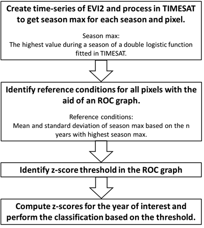
Fig. 3. Workflow of the developed defoliation detection method. The 2-band Enhanced Vegetation Index (EVI2) is derived from MODIS data with 250 m spatial and 8 days temporal resolution, and smoothed with double logistic functions in the TIMESAT software (Jönsson and Eklundh 2002, 2004). Receiver Operating Characteristics (ROC) graphs are used to visualize the ratio of the damaged MODIS pixels that were correctly classified and the ratio of healthy MODIS pixels that are misclassified as damaged. The number of years to base the reference condition on and the z-score threshold were decided based on the ROC graph.
2.3.4 Evaluation and generalization
Evaluation data were divided into two areas: (1) Outokumpu, with a short history of insect defoliation, and (2) Ilomantsi, where the insect infestation has been persistent during the entire time-series of MODIS data. Evaluation was then performed with the threshold identified in the training data.
The method was also applied to the sampling units in Abisko: Time-series of EVI2 with a temporal resolution of eight days were created for the years 2001–2013. ROC curves were computed as for Outokumpu and plotted to find the optimal number of years to base the reference conditions on, and to find the z-score threshold. In Abisko all field data were used as training data to get more data to support the ROC graph.
3 Results
3.1 ROC curves and evaluation
Receiver Operating Characteristics curves for EVI2 computed from the training data in Outokumpu are shown in Fig. 4. They show that when reference conditions are estimated from four (ROC4) and five (ROC5) years, the curves are similar, and identical at the optimal threshold (z = –2.9). The ROC curve for six years (ROC6) is lower, i.e. more healthy observations are classified as damaged. ROC7 is lower than ROC6 and omitted in the figure for reasons of legibility. Since we considered it more statistically robust to base the reference conditions on five years than four, the reference conditions were estimated from the five years with highest season max. The optimal z-score threshold for our purpose is at –2.9, which resulted in 50% of the damaged plots being detected with no misclassification of healthy plots (Fig. 4). When the training data were classified into damaged and healthy observations with a defoliation threshold of 25%, a z-score threshold of –4.5 resulted in 61% of the damaged pixels being detected with a misclassification of healthy pixels of 6%. A defoliation threshold of 15% resulted in accuracies identical to the 20% threshold. This suggests that the defoliation threshold did not have a major influence on the detection accuracy. Since the evaluation data were classified into damaged and healthy with a threshold of 20% no evaluation could be performed with the other defoliation thresholds.
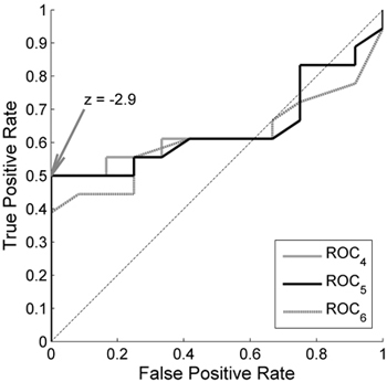
Fig. 4. Receiver Operating Characteristics (ROC) curves for the 2-band Enhanced Vegetation Index (EVI2) in Outokumpu. True Positive Rate is the ratio of the damaged MODIS pixels that were classified as damaged, and False Positive Rate is the ratio of the healthy pixels that were classified as damaged. A single curve is created by applying the developed method with the damage detection based on a range of different z-score thresholds. The different curves are created by basing the reference conditions on the 4 years (ROC4), 5 years (ROC5) and 6 years (ROC6) with highest season max values. z = –2.9 is the threshold that gives a result closest to the theoretically best classification at coordinate (0,1).
Receiver Operating Characteristics curves for NDVI (Fig. 5) show a zig-zag pattern suggesting that it is not obvious what number of years to base the reference conditions on, and that there is no obvious optimal z-score threshold. For lower TPR (~0.25) the classification is more or less random; for higher thresholds the ROC curves are nearly parallel to the diagonal. Hence, the most suitable threshold strongly depends on the purpose of a study. Since NDVI results in extensive misclassification of healthy plots for low TPR, EVI2 was the preferred index in this study. However, if the main purpose of a study is to detect defoliation, and misclassification of healthy stands is to a larger degree acceptable, NDVI may be more suitable.
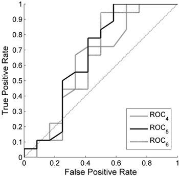
Fig. 5. Receiver Operating Characteristics (ROC) curves for the Normalized Difference Vegetation Index (NDVI) in Outokumpu. True Positive Rate is the ratio of the damaged MODIS pixels that were classified as damaged, and False Positive Rate is the ratio of the healthy pixels that were classified as damaged. A single curve is created by applying the developed method with the damage detection based on a range of different z-score thresholds. The different curves are created by basing the reference conditions on the 4 years (ROC4), 5 years (ROC5) and 6 years (ROC6) with highest season max values. z = –2.9 is the threshold that gives a result closest to the theoretically best classification at coordinate (0,1).
The method was evaluated by applying the z-score thresholds for EVI2 to the evaluation data. In Outokumpu, with a shorter history of insect infestation, 50% of the defoliated evaluation stands were detected with a misclassification of healthy stands of 22% (Table 2). In Ilomantsi, with a long history of insect infestation, the method was not successful; only 27% of the damaged stands were detected with a misclassification of 54%. These results indicate the importance of years with satellite data available for a number of years prior to an outbreak to enable identification of reference conditions. To illustrate the ability to adjust the z-score threshold to tailor the method to a specific purpose, we also applied a higher (z = –2.1) threshold that resulted in 50% misclassification of healthy stands in the training data. In the evaluation data this threshold resulted in 63% of the damaged stands being detected with a misclassification of healthy stands of 37% in Outokumpu. In Ilomantsi, the higher threshold resulted in 46% damaged stands detected with a 70% misclassification of healthy stands.
| Table 2. Results of the method evaluation for the Outokumpu and Ilomantsi areas. Thresholds are z-scores of the seasonal maximum of the 2-band Enhanced Vegetation Index (EVI2) fitted to a double logistic function in TIMESAT. The lower threshold is the threshold that gave a classification closest to the theoretically perfect classification, while the higher threshold is a threshold that resulted in 50% misclassification of healthy pixels in the training data. | ||||
| Outokumpu | Ilomantsi | |||
| Threshold (EVI2 z-score) | –2.9 | –2.1 | –2.9 | –2.1 |
| Detected defoliation | 50% | 63% | 27% | 46% |
| Misclassified healthy stands | 22% | 37% | 54% | 70% |
3.2 Method generalization
The Receiver Operating Characteristics graph for Abisko suggests that the reference conditions should be based on six years and the threshold should be set to z = –6.0 (Fig. 6). ROC curves based on fewer or more years are closer to the diagonal. The point closest to (0,1) for ROC6 is at TPR = 0.75 and FPR = 0.19. This suggests that 75% of the damage can be detected with a misclassification of healthy sampling units of 19%. These considerably better results indicate that MODIS data perform better in the natural and more homogenous forest landscapes in Abisko.
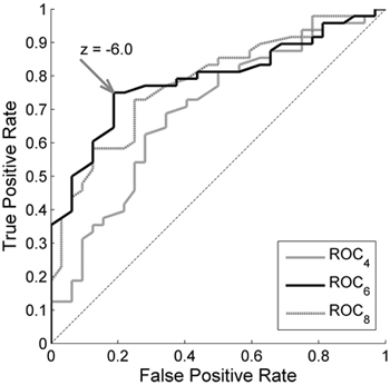
Fig. 6. Receiver Operating Characteristics (ROC) curves for the 2-band Enhanced Vegetation Index (EVI2) in Abisko. True Positive Rate is the ratio of the damaged MODIS pixels that were classified as damaged, and False Positive Rate is the ratio of the healthy pixels that were classified as damaged. A single curve is created by applying the developed method with the damage detection based on a range of different z-score thresholds. The different curves are created by basing the reference conditions on the 4 years (ROC4), 6 years (ROC6) and 8 years (ROC8) with highest season max values. z = –2.9 is the threshold that gives a result closest to the theoretically best classification at coordinate (0,1).
4 Discussion
4.1 Factors affecting detection accuracy
This study has indicated both possibilities and difficulties in using low spatial resolution data for monitoring of insect induced defoliation in Fennoscandian forests. In the more homogenous natural area in northern Sweden the method was successful and detected 75% of the damaged sampling units with a misclassification of healthy units of 19%. In the fragmented and heavily managed forest landscapes in Finland with small individual forest stands the accuracies were lower with 50–63% of the defoliation detected and with a misclassification of healthy stands of 22–37%. Where the history of the insect outbreak was long, as in Ilomantsi, the method resulted in extensive misclassification rates. The main reason for the limitation in the fragmented areas is most likely the low spatial resolution of MODIS, which results in mixed pixels that may contain both healthy and damaged forest stands. The detection accuracies in Finland are lower than in a study conducted in Ilomantsi with Landsat TM images, where Ilvesniemi (2009) reached a classification accuracy of 85.9% for two defoliation classes. These results are also generally lower than corresponding studies using MODIS in more homogeneous forest areas in North America (de Beurs and Townsend 2008) and Russia (Kharuk et al. 2007). However, the high detection accuracies observed in Abisko show that the developed method does enable defoliation detection in other forest types.
The outbreak history also influences the detection accuracy, as noted by Sulla-Menashe et al. (2014) who concluded that a history of forest disturbances influences the ability to detect present disturbance events. In Ilomantsi the accuracy was poor, mainly as a consequence of recurring insect attacks during the entire time period studied, and the associated difficulty in establishing stable reference conditions. In Outokumpu, where the MODIS record was long enough to establish stable reference conditions, results were more accurate (50% of the damage detected with 22% false alarm). It is likely that the main problem is that the foliage in the pine forests does not fully recover between insect outbreaks. Growth recovery after an attack may continue over a time period of 5−10 years (Lyytikäinen-Saarenmaa and Tomppo 2002). Hence, the years with low defoliation are still influenced by previous defoliation events, and the reference conditions will be based on recovering rather than healthy forest. In the deciduous forests in Abisko the situation is different. Even though the birch forests require long periods of recovery; after an outbreak in Abisko 1954−55 the forests had regained only 75% of the pre-outbreak biomass as late as in 1987 (Tenow 1996), we observed that the foliage regains sufficient leaf area to return to pre-outbreak levels of EVI2 already the year after an outbreak. Hence, reference conditions could be established despite the fact that there were insect outbreaks present in the available time-series of MODIS data. These results also indicate that in areas with frequent insect attacks coniferous forests are more difficult to monitor than deciduous forests. Furthermore, it is quite likely that the severity of the defoliation influences the ability to monitor an outbreak. In Abisko, and in the study of pine sawfly attacks by Eklundh et al. (2009) that resulted in high detection accuracies (82%), large areas were almost totally defoliated. In Finland, on the other hand, defoliation intensities were more fluctuating and generally less severe.
Other factors, such as the timings of defoliation events, may also affect the detection accuracy. In Outokumpu the larval period of the European pine sawfly took place early in June (Lyytikäinen-Saarenmaa 1999). Also in Abisko the defoliation occurred in the early summer (Tenow et al. 2007). In Ilomantsi, on the other hand, the defoliation was caused by the common pine sawfly having a larval period later, in July–September (Lyytikäinen-Saarenmaa 1999), i.e. well after the season max. In addition, in late summer, solar elevation angles are lower, resulting in more shadows and bi-directional scattering effects, which influence the remotely sensed reflectances, and hence, vegetation indices.
4.2 Z-score classification and season max
We used z-scores in order to develop a method that is adaptive to the natural variability of the satellite data. It could be argued that a one-tailed t-test could be applied instead and that this might have the advantage of being less site-specific. However, since the method is applied pixel-wise we considered the amount of data too low to estimate robust mean values and standard deviations to apply a t-test at a specific significance level. In addition, z-scores allows utilizing ROC curves to decide the threshold for disturbance detection, which allows a user to weight the trade-off between disturbance detection and false alarm to suit the purpose of a study. Furthermore, we anticipate that the z-score thresholds can be applied for similar land cover over extensive areas and that the thresholds are land cover specific rather than site-specific. The method does, however, require that land cover data are available to identify which MODIS pixels to monitor.
Season max was used as a metric for forest health to detect defoliation in this study. The motivation is that season max is a robust parameter since it is based on all data from a season, weighted according to data quality, and thereby less sensitive to noise and low quality data. Another advantage with season max is that it makes the method less sensitive to phenological variability; season max from different seasons can be directly compared without any need to identify the start of the growing season. In addition, season max makes the method more general since the same metric can be applied to monitor outbreaks regardless of the defoliation period of the insect studied. During the method development we made tentative visual tests with mean values for shorter periods, where the periods were chosen to coincide with the main defoliation period of the insect studied. These tests did not perform better than z-scores of season max. However, a high value of season max after an outbreak might be due to other reasons than recovering forests, such as understory vegetation development favoured by improved light conditions, and should not be considered as recovered trees per se. For a disturbance monitoring method this is likely to be less of a problem, since the main aim is to detect the defoliation event in the first place.
4.3 Implications for developing a forest defoliation monitoring system and future satellite data
Given the variation in accuracies achieved in this study and the fact that high spatial resolution satellite data generally are more accurate, the role of low-resolution systems in forest disturbance monitoring can be discussed. While considering their weaknesses, these low spatial resolution systems do have advantages in terms of more frequent coverage in time, low computational demand, and historical continuity in time. Consequently, low spatial resolution data may have a role to play in regional and global forest disturbance monitoring, especially in areas where cloudy conditions limits the number of available medium-resolution images, and where a short growing season limits the number of potentially available medium-resolution images. As an example, only small fractions of the study area in Abisko were visible in any Landsat image during the outbreak in 2013. However, it must be realized that in areas with fragmented forest landscapes low-resolution data results in low detection accuracies, and where the disturbance history is longer than the satellite time-series record, damage might be undetected. Forest conditions similar to those in Finland are common elsewhere in Fennoscandia, but also not uncommon elsewhere in the world. Hence, it is quite likely that forest damage based on MODIS data in these areas is underestimated. Therefore, if there is a sufficient number of medium-resolution images available during the main growing season these data should be preferred.
One possibility to reduce the limitation of the low spatial resolution of MODIS could be to apply data fusion methods, such as the Spatial and Temporal Adaptive Reflectance Fusion Model (STARFM) (Gao et al. 2006) and the Enhanced STARFM (ESTARFM) (Zhu et al. 2010) that were developed to combine e.g. Landsat and MODIS data. Both STARFM and ESTARFM enable creation of images with high temporal and spatial resolution; however, they cannot detect ephemeral disturbances with high accuracy if the disturbance is not registered in any of the Landsat images utilized (Zhu et al. 2010). The Temporal Adaptive Algorithm for mapping Reflectance Change (STAARCH) is a data fusion method that was developed for disturbance detection (Hilker et al. 2009). STAARCH enables detection of disturbances such as clear cuts and fires with high accuracy, but has limitations in detecting short-term transient disturbances such as insect outbreaks since the detection of spatial change mainly relies on Landsat, while MODIS data are applied to identify the timing of disturbances. Hence, the ability of data fusion methods to detect insect defoliation events to a large extent depends on the ability of MODIS data to detect the damage in areas with frequent cloud cover.
With the launch of the first Sentinel-2 satellite in 2015 and the planned launch of the second satellite in 2016 (ESA 2015a), the possibilities to detect damage in fragmented forests is likely to be improved. These satellites, carrying the Multi Spectral Instrument (MSI), will have the advantage of high spatial resolution (10−60 m) and high temporal resolution, with a revisit time of 5 days at the equator (Drusch et al. 2012) and 2−3 days at mid-latitudes (ESA 2015a). The high spatial resolution will substantially decrease the number of mixed pixels, and the high temporal resolution may turn out to be sufficient for modelling the seasonal trajectory for each pixel and to detect insect defoliation. In addition, Sentinel-2 MSI provides 13 spectral bands (Drusch et al. 2012) which open up for the possibility to monitor forest disturbances with a wide range of vegetation indices that might further improve detection accuracy. For example, indices including shortwave infrared (SWIR) wavelength bands derived from Landsat data have been successful for accurate detection of insect defoliation (Skakun et al. 2003; Wang et al. 2007; Goodwin et al. 2008; Coops et al. 2010). In principle, the z-score method is well suited also to these band combinations and to high spatial resolution data. If the lower temporal resolution of Sentinel-2 compared to MODIS will be a limitation in Fennoscandia remains to be tested, however, opportunities exist to merge the data with Landsat-8 to increase the temporal resolution. The z-score method developed in this study requires that the reference conditions can be estimated also for Sentinel-2 MSI pixels, which implies that Sentinel-2 data must be available for several years before the methods can be applied, and that these years are not influenced by disturbances. An alternative approach would be to apply data fusion methods to derive reference conditions based on MODIS and higher spatial resolution data to establish the reference condition also based on presently available data.
5 Conclusions
The results of this study indicate difficulties in relying solely on MODIS data for a general insect damage detection system over fragmented Fennoscandian forest landscapes. The coarse-resolution satellite data can provide high as well as low accuracies, and may fail entirely to detect damage in very heterogeneous forests. The problem is aggravated when the damage history is very long, as in one of our study areas. Therefore, studies of defoliation based on these data may underestimate defoliation damage in Fennoscandia and similar forest types. However, MODIS and other low-resolution satellite data may still have an important role to play in disturbance monitoring, especially in regions where cloudy conditions limits the number of available medium-resolution images. In addition, the developed method based on TIMESAT, z-scores and ROC curves developed in this paper is robust, and succeeded in detecting defoliation events with high accuracy in the more homogenous forests in Abisko. Hence, it might be possible to apply the developed method to other future satellite data. Sentinel-2 MSI data with its high spatial, spectral and temporal resolutions is particularly interesting for future monitoring of forest disturbances.
Acknowledgements
This project was mainly funded by a research grant from the Swedish National Space Board. We also received financial aid from the Niemi foundation, the Maj and Tor Nessling Foundation, and the Finnish Academy project ‘Centre of Excellence in Laser Scanning Research’ (CoE-LaSR, decision number 272195). We wish to thank Antero Pasanen, Jari Tahvanainen and Taisto Saarelainen from Tornator Ltd. for enabling the study at the Palokangas and Outokumpu areas. We also thank Minna Blomqvist, Maiju Kosunen, and Mervi Talvitie for collecting the field data with us, and Annika Kristoffersson at Abisko Scientific Research Station for providing us with temperature data. We also acknowledge the Land Processes Distributed Active Archive Center (LP DAAC) for providing access to the MODIS data, as well as the E-OBS dataset from the EU-FP6 project ENSEMBLES (http://ensembles-eu.metoffice.com) and the data providers in the ECA&D project (http://www.ecad.eu).
References
Abisko Scientific Research Station (2015). Temperature data, 1913–2014. http://www.polar.se/abisko.
Adelabu S., Mutanga O., Cho M.A. (2012). A review of remote sensing of insect defoliation and its implications for the detection and mapping of Imbrasia belina defoliation of Mopane Woodland. The African Journal of Plant Science and Biotechnology 6: 1–13.
Anees A., Aryal J. (2014). Near-real time detection of beetle infestation in pine forests using MODIS data. IEEE Journal of Selected Topics in Applied Earth Observations and Remote Sensing 7: 3713–3723. http://dx.doi.org/10.1109/JSTARS.2014.2330830.
Babst F., Esper J., Parlow E. (2010). Landsat TM/ETM+ and tree-ring based assessment of spatiotemporal patterns of the autumnal moth (Epirrita autumnata) in northernmost Fennoscandia. Remote Sensing of Environment 114: 637–646. http://dx.doi.org/10.1016/j.rse.2009.11.005.
Björkman C., Bylund H., Klapwijk M.J., Kollberg I., Schroeder M. (2011). Insect pests in future forests: more severe problems? Forests 2: 474–485. http://dx.doi.org/10.3390/f2020474.
Bylund H. (1995). Long-term interactions between the autumnal moth and mountain birch: the role of resources, competitors, natural enemies, and weather. Ph.D. thesis, Swedish University of Agricultural Sciences, Uppsala.
Cajander A.K. (1926). The theory of forest types. Acta Forestalia Fennica 29: 1–108.
Callaghan T.V., Bergholm F., Christensen T.R., Jonasson C., Kokfelt U., Johansson M. (2010). A new climate era in the sub-Arctic: accelerating climate changes and multiple impacts. Geophysical Research Letters 37: L14705. http://dx.doi.org/10.1029/2009GL042064.
Cohen W.B., Yang Z., Kennedy R. (2010). Detecting trends in forest disturbance and recovery using yearly Landsat time series: 2. TimeSync – tools for calibration and validation. Remote Sensing of Environment 114: 2911–2924. http://dx.doi.org/10.1016/j.rse.2010.07.010.
Coops N.C., Gillanders S.N., Wulder M.A., Gergel S.E., Nelson T., Goodwin N.R. (2010). Assessing changes in forest fragmentation following infestation using time series Landsat imagery. Forest Ecology and Management 259: 2355–2365. http://dx.doi.org/10.1016/j.foreco.2010.03.008.
de Beurs K.M., Townsend P.A. (2008). Estimating the effect of gypsy moth defoliation using MODIS. Remote Sensing of Environment 112: 3983−3990. http://dx.doi.org/10.1016/j.rse.2008.07.008.
De Somviele B., Lyytikäinen-Saarenmaa P., Niemelä P. (2007). Stand edge effects on distribution and condition of Diprionid sawflies. Agricultural and Forest Entomology 9: 17–30. http://dx.doi.org/10.1111/j.1461-9563.2006.00313.x.
Dix M.E., Buford M., Slavicek J., Solomon A.M., Conrad S.G. (2009). Invasive species and disturbances: current and future roles of Forest Service research and development. A dynamic invasive species research vision 29: 91–102.
Drusch M., Del Bello U., Carlier S., Colin O., Fernandez V., Gascon F., Hoersch B., Isola C., Laberinti P., Martimort P., Meygret A., Spoto F., Sy O., Marchese F., Bargellini P. (2012). Sentinel-2: ESA’s optical high-resolution mission for gmes operational services. Remote Sensing of Environment 120: 25–36. http://dx.doi.org/10.1016/j.rse.2011.11.026.
Eichhorn J. (1998). Manual on methods and criteria for harmonized sampling, assessment, monitoring and analysis of the effects of air pollution on forests. Part II. Visual assessment of crown condition and submanual on visual assessment of crown condition on intensive monitoring plots. United Nations Economic Commission for Europe Convention on Long-Range Transboundary Air Pollution, Hamburg, Germany.
Eklundh L., Johansson T., Solberg S. (2009). Mapping insect defoliation in Scots pine with MODIS time-series data. Remote Sensing of Environment 113: 1566–1573. http://dx.doi.org/10.1016/j.rse.2009.03.008.
ESA (2015a). ESA: Sentinel-2. http://www.esa.int/Our_Activities/Observing_the_Earth/Copernicus/Sentinel-2/Introducing_Sentinel-2. [Cited 16 Dec 2015].
ESA (2015b). ESA Earth Online: Sentinel-3. https://earth.esa.int/web/guest/missions/esa-future-missions/sentinel-3. [Cited 16 Dec 2015].
Fawcett T. (2006). An introduction to ROC analysis. Pattern Recognition Letters 27: 861–874. http://dx.doi.org/10.1016/j.patrec.2005.10.010.
Franklin S., Wulder M., Skakun R., Carroll A. (2003). Mountain pine beetle red attack damage classification using stratified Landsat TM data in British Columbia, Canada. Photogrammetric Engineering and Remote Sensing 69: 283–288. http://dx.doi.org/10.14358/PERS.69.3.283.
Fraser R.H., Abuelgasim A., Latifovic R. (2005). A method for detecting large-scale forest cover change using coarse spatial resolution imagery. Remote Sensing of Environment 95: 414–427. http://dx.doi.org/10.1016/j.rse.2004.12.014.
Gao F., Masek J., Schwaller M., Hall F. (2006). On the blending of the landsat and MODIS surface reflectance: predicting daily landsat surface reflectance. IEEE Transactions on Geoscience and Remote Sensing 44: 2207–2218. http://dx.doi.org/10.1109/TGRS.2006.872081.
Gitelson A. (2004). Wide dynamic range vegetation index for remote quantification of biophysical characteristics of vegetation. Journal of Plant Physiology 161: 165–173. http://dx.doi.org/10.1078/0176-1617-01176.
Goodwin N.R., Coops N.C., Wulder M.A., Gillanders S., Schroeder T.A., Nelson T. (2008). Estimation of insect infestation dynamics using a temporal sequence of Landsat data. Remote Sensing of Environment 112: 3680–3689. http://dx.doi.org/10.1016/j.rse.2008.05.005.
Hansen M.C., Potapov P.V., Moore R., Hancher M., Turubanova S.A., Tyukavina A., Thau D., Stehman S.V., Goetz S.J., Loveland T.R., Kommareddy A., Egorov A., Chini L., Justice C.O., Townshend J.R.G. (2013). High-resolution global maps of 21st-century forest cover change. Science 342: 850–853. http://dx.doi.org/10.1126/science.1244693.
Haylock M.R., Hofstra N., Klein Tank A.M.G., Klok E.J., Jones P.D., New M. (2008). A European daily high-resolution gridded dataset of surface temperature and precipitation. Journal of Geophysical Research (Atmospheres) 113: D20119. http://dx.doi.org/10.1029/2008JD10201.
Heliasz M., Johansson T., Lindroth A., Mölder M., Mastepanov M., Friborg T., Callaghan T.V., Christensen T.R. (2011). Quantification of C uptake in subarctic birch forest after setback by an extreme insect outbreak. Geophysical Research Letters 38: L01704. http://dx.doi.org/10.1029/2010GL044733.
Hilker T., Wulder M.A., Coops N.C., Linke J., McDermid G., Masek J.G., Gao F., White J.C. (2009). A new data fusion model for high spatial- and temporal-resolution mapping of forest disturbance based on Landsat and MODIS. Remote Sensing of Environment 113: 1613–1627. http://dx.doi.org/10.1016/j.rse.2009.03.007.
Hlásny T., Zajičková L., Turčáni M., Holuša J., Sitková Z. (2011). Geographical variability of Spruce bark beetle development under climate change in the Czech Republic. Journal of Forest Science 57: 242–249.
Huete A., Didan K., Miura T., Rodriguez E.P., Gao X., Ferreira L.G. (2002). Overview of the radiometric and biophysical performance of the MODIS vegetation indices. Remote Sensing of Environment 83: 195–213. http://dx.doi.org/10.1016/S0034-4257(02)00096-2.
Huete A.R., Liu H.Q., Batchily K., van Leeuwen W. (1997). A comparison of vegetation indices over a global set of TM images for EOS-MODIS. Remote Sensing of Environment 59: 440–451. http://dx.doi.org/10.1016/S0034-4257(96)00112-5.
Ilvesniemi S. (2009). Numeeriset ilmakuvat ja Landsat TM-satelliittikuvat männyn neulaskadon arvioinnissa. [Detecting defoliation with digital aerial phots and Landsat TM data]. Helsingin yliopisto, Helsinki, Finland. p. 62.
Jepsen J.U., Hagen S.B., Ims R.A., Yoccoz N.G. (2008). Climate change and outbreaks of the geometrids Operophtera brumata and Epirrita autumnata in subarctic birch forest: evidence of a recent outbreak range expansion. Journal of Animal Ecology 77: 257–264. http://dx.doi.org/10.1111/j.1365-2656.2007.01339.x.
Jepsen J.U., Hagen S.B., Høgda K.A., Ims R.A., Karlsen S.R., Tømmervik H., Yoccoz N.G. (2009). Monitoring the spatio-temporal dynamics of geometrid moth outbreaks in birch forest using MODIS-NDVI data. Remote Sensing of Environment 113: 1939–1947. http://dx.doi.org/10.1016/j.rse.2009.05.006.
Jiang Z., Huete A.R., Didan K., Miura T. (2008). Development of a two-band enhanced vegetation index without a blue band. Remote Sensing of Environment 112: 3833–3845. http://dx.doi.org/10.1016/j.rse.2008.06.006.
Jönsson P., Eklundh L. (2002). Seasonality extraction by function fitting to time-series of satellite sensor data. IEEE Transactions on Geoscience and Remote Sensing 40(8): 1824–1832. http://dx.doi.org/10.1109/TGRS.2002.802519.
Jönsson P., Eklundh L. (2004). TIMESAT-a program for analyzing time-series of satellite sensor data. Computers & Geosciences 30: 833–845. http://dx.doi.org/10.1016/j.cageo.2004.05.006.
JPSS (2015). About JPSS: Visible Infrared Imaging Radiometer Suite (VIIRS). JPSS. http://www.jpss.noaa.gov/viirs.html. [Cited 16 Dec 2015].
Kantola T., Vastaranta M., Yu X., Lyytikäinen-Saarenmaa P., Holopainen M., Talvitie M., Kaasalainen S., Solberg S., Hyyppä J. (2010). Classification of defoliated trees using tree-level airborne laser scanning data combined with aerial images. Remote Sensing 2: 2665–2679. http://dx.doi.org/10.3390/rs2122665.
Kennedy R.E., Yang Z., Cohen W.B. (2010). Detecting trends in forest disturbance and recovery using yearly Landsat time series: 1. LandTrendr - temporal segmentation algorithms. Remote Sensing of Environment 114: 2897–2910. http://dx.doi.org/10.1016/j.rse.2010.07.008.
Kharuk V.I., Ranson K.J., Kozuhovskaya A.G., Kondakov Y.P., Pestunov I.A. (2004). NOAA/AVHRR satellite detection of Siberian silkmoth outbreaks in eastern Siberia. International Journal of Remote Sensing 25: 5543–5556.
Kharuk V.I., Ranson K.J., Fedotova E.V. (2007). Spatial pattern of Siberian silkmoth outbreak and taiga mortality. Scandinavian Journal of Forest Research 22: 531–536. http://dx.doi.org/10.1080/02827580701763656.
Kharuk V.I., Ranson K.J., Im S.T. (2009). Siberian silkmoth outbreak pattern analysis based on SPOT VEGETATION data. Remote Sensing of Environment 30: 2377–2388. http://dx.doi.org/10.1080/01431160802549419.
Kurz W.A., Stinson G., Rampley G. (2008). Could increased boreal forest ecosystem productivity offset carbon losses from increased disturbances? Philosophical Transactions of the Royal Society of London B: Biological Sciences 363: 2259–2268. http://dx.doi.org/10.1098/rstb.2007.2198.
Lindner M., Maroschek M., Netherer S., Kremer A., Barbati A., Garcia-Gonzalo J., Seidl R., Delzon S., Corona P., Kolström M., Lexer M.J., Marchetti M. (2010). Climate change impacts, adaptive capacity, and vulnerability of European forest ecosystems. Forest Ecology and Management 259: 698–709. http://dx.doi.org/10.1016/j.foreco.2009.09.023.
Linke J., Betts M.G., Lavigne M.B., Franklin S.E. (2007). Introduction: structure, function, and change of forest landscapes. In: Wulder M.A., Franklin S.E. (eds.). Understanding forest disturbance and spatial pattern. CRC Press, Taylor and Francis Group, Boca Raton, FL, USA. p. 1–29.
Logan J.A., Regniere J., Powell J.A. (2003). Assessing the impacts of global warming on forest pest dynamics. Frontiers in Ecology and the Environment 1: 130–137. http://dx.doi.org/10.1890/1540-9295(2003)001[0130:ATIOGW]2.0.CO;2.
LPDAAC (2012a). Surface Reflectance 8-Day L3 Global 250m, Land Processes Distributed Active Archive Center. https://lpdaac.usgs.gov/dataset_discovery/modis/modis_products_table/mod09q1.
LPDAAC (2012b). Surface Reflectance 8-Day L3 Global 500m, Land Processes Distributed Active Archive Center. https://lpdaac.usgs.gov/dataset_discovery/modis/modis_products_table/mod09a1.
LPDAAC (2012c). Vegetation Indices 16-Day L3 Global 250m, Land Processes Distributed Active Archive Center. https://lpdaac.usgs.gov/dataset_discovery/modis/modis_products_table/mod13q1.
LPDAAC (2012d). MODIS Overview, Land Processes Distributed Active Archive Center. https://lpdaac.usgs.gov/dataset_discovery/modi.
Lyytikäinen-Saarenmaa P. (1999). Growth responses of Scots pine (Pinaceae) to artificial and sawfly (Hymenoptera: Diprionidae) defoliation. Canadian Entomologist 131: 455–463. http://dx.doi.org/10.4039/Ent131455-4.
Lyytikäinen-Saarenmaa P., Tomppo E. (2002). Impact of sawfly defoliation on growth of Scots pine Pinus sylvestris (Pinaceae) and associated economic losses. Bulletin of Entomological Research 92: 137–140. http://dx.doi.org/10.1079/BER2002154.
Lyytikäinen-Saarenmaa P., Holopainen M., Ilvesniemi S., Haapanen R. (2008). Detecting pine sawfly defoliation by means of remote sensing and GIS. Forstschutz Aktuell 44: 14–15.
Meigs G.W., Kennedy R.E., Cohen W.B. (2011). A Landsat time series approach to characterize bark beetle and defoliator impacts on tree mortality and surface fuels in conifer forests. Remote Sensing of Environment 115: 3707–3718. http://dx.doi.org/10.1016/j.rse.2011.09.009.
Melaas E.K., Friedl M.A., Zhu Z. (2013). Detecting interannual variation in deciduous broadleaf forest phenology using Landsat TM/ETM + data. Remote Sensing of Environment 132: 176–185. http://dx.doi.org/10.1016/j.rse.2013.01.011.
Netherer S., Schopf A. (2012). Potential effects of climate change on insect herbivores in European forests-General aspects and the pine processionary moth as specific example. Forest Ecology and Management 259: 831–838. http://dx.doi.org/10.1016/j.foreco.2009.07.034.
Olsson P.O., Jönsson A.M., Eklundh L. (2012). A new invasive insect in Sweden - Physokermes inopinatus: tracing forest damage with satellite based remote sensing. Forest Ecology and Management 285: 29–37. http://dx.doi.org/10.1016/j.foreco.2012.08.003.
Peters A.J., WalterShea E.A., Lel J., Vliia A., Hayes M., Svoboda M.D. (2002). Drought monitoring with NDVI-based standardized vegetation index. Photogrammetric Engineering and Remote Sensing 68: 71–75.
Rouse J.W., Haas R.H., Shell J.A., Deering D.W. (1973). Monitoring vegetation systems in the Great Plains with ERTS-1. Third ERTS Symposium, NASA SP-351 I. p. 309–317.
Rullan-Silva C.D., Olthoff A.E., Delgado de la Mata J.A., Pajares-Alonso J.A. (2013). Remote monitoring of forest insect defoliation - a review. Forest Systems 22: 377–391. http://dx.doi.org/10.5424/fs/2013223-04417.
Skakun R.S., Wulder M.A., Franklin S.E. (2003). Sensitivity of the thematic mapper enhanced wetness difference index to detect mountain pine beetle red-attack damage. Remote Sensing of Environment 86: 433–443. http://dx.doi.org/10.1016/S0034-4257(03)00112-3.
Spruce J.P., Sader S., Ryan R.E., Smoot J., Kuper P., Ross K., Prados D., Russell J., Gasser G., McKellip R., Hargrove W. (2011). Assessment of MODIS NDVI time series data products for detecting forest defoliation by gypsy moth outbreaks. Remote Sensing of Environment 115: 427–437. http://dx.doi.org/10.1016/j.rse.2010.09.013.
Sulla-Menashe D., Kennedy R.E., Yang Z., Braaten J., Krankina O.N., Friedl M.A. (2014). Detecting forest disturbance in the Pacific Northwest from MODIS time series using temporal segmentation. Remote Sensing of Environment 151: 114–123. http://dx.doi.org/10.1016/j.rse.2013.07.042.
Talvitie M., Kantola T., Holopainen M., Lyytikäinen-Saarenmaa P. (2011). Adaptive cluster sampling in inventorying forest damage by the Common pine sawfly (Diprion pini). Journal of Forest Planning 16:1–7.
Tan B., Woodcock C.E., Hu J., Zhang P., Ozdogan M., Huang D., Yang W., Knyazikhin Y., Myneni R.B. (2006). The impact of gridding artifacts on the local spatial properties of MODIS data: implications for validation, compositing, and band-to-band registration across resolutions. Remote Sensing of Environment 105: 98–114. http://dx.doi.org/10.1016/j.rse.2006.06.008.
Tenow O. (1996). Hazards to a mountain birch forest: Abisko in perspective. Ecological Bulletins 104–114. http://www.jstor.org/stable/20113188.
Tenow O., Nilssen A. (1990). Egg cold hardiness and topoclimatic limitations to outbreaks of Epirrita autumnata in northern Fennoscandia. Journal of Applied Ecology 27: 723–734. http://dx.doi.org/10.2307/2404314.
Tenow O., Nilssen A.C., Bylund H., Hogstad O. (2007). Waves and synchrony in Epirrita autumnata /Operophtera brumata outbreaks. I. Lagged synchrony: regionally, locally and among species. Journal of Animal Ecology 76: 258–268. http://dx.doi.org/10.1111/j.1365-2656.2006.01204.x.
Townshend J.R., Masek J.G., Huang C., Vermote E.F., Gao F., Channan S., Sexton J.O., Feng M., Narasimhan R., Kim D., Song K., Song D., Song X.-P., Noojipady P., Tan B., Hansen M.C., Li M., Wolfe R.E. (2012). Global characterization and monitoring of forest cover using Landsat data: opportunities and challenges. International Journal of Digital Earth 5: 373–397. http://dx.doi.org/10.1080/17538947.2012.713190.
Townshend J.R.G., Huang C., Kalluri S.N.V., Defries R.S., Liang S., Yang K. (2000). Beware of per-pixel characterization of land cover. International Journal of Remote Sensing 21: 839–843.
Tucker C.J. (1979). Red and photographic infrared linear combinations for monitoring vegetation. Remote Sensing of Environment 8: 127–150. http://dx.doi.org/10.1016/0034-4257(79)90013-0.
Vanhanen H., Veteli T.O., Päivinen S., Kellomäki S., Niemelä P. (2007). Climate change and range shifts in two insect defoliators: gypsy moth and nun moth – a model study. Silva Fennica 41(4): 621–638. http://dx.doi.org/10.14214/sf.469.
Vermote E.F., Kotchenova S.Y., Ray J.P. (2011). MODIS Surface Reflectance user’s guide, version 1.3. MODIS Land Surface Reflectance Science Computing. http://modis-sr.ltdri.org/guide/MOD09_UserGuide_v1_3.pdf.
Wang C., Lu Z., Haithcoat T.L. (2007). Using Landsat images to detect oak decline in the Mark Twain National Forest, Ozark Highlands. Forest Ecology and Management 240: 70–78. http://dx.doi.org/10.1016/j.foreco.2006.12.007.
Wang D., Morton D., Masek J., Wu A., Nagol J., Xiong X., Levy R., Vermote E., Wolfe R. (2012). Impact of sensor degradation on the MODIS NDVI time series. Remote Sensing of Environment 119: 55–61. http://dx.doi.org/10.1016/j.rse.2011.12.001.
Wielgolaski F.E. (2001). Vegetation sections in northern Fennoscandian mountain birch forest. In: Wielgolaski F.E. (ed.). Nordic mountain birch ecosystems. The Parthenon Publishing Group, London. p. 23–46.
Wulder M.A., Dymond C.C., White J.C., Leckie D.G., Carroll A.L. (2006). Surveying mountain pine beetle damage of forests: a review of remote sensing opportunities. Forest Ecology and Management 221: 27–41. http://dx.doi.org/ 10.1016/j.foreco.2005.09.021.
Wulder M.A., Masek J.G., Cohen W.B., Loveland T.R., Woodcock C.E. (2012). Opening the archive: how free data has enabled the science and monitoring promise of Landsat. Remote Sensing of Environment 122: 2–10. http://dx.doi.org/10.1016/j.rse.2012.01.010.
Zhu X., Chen J., Gao F., Chen X., Masek J.G. (2010). An enhanced spatial and temporal adaptive reflectance fusion model for complex heterogeneous regions. Remote Sensing of Environment 114: 2610–2623. http://dx.doi.org/10.1016/j.rse.2010.05.032.
Zhu Z., Woodcock C.E., Olofsson P. (2012). Continuous monitoring of forest disturbance using all available Landsat imagery. Remote Sensing of Environment 122: 75–91. http://dx.doi.org/10.1016/j.rse.2011.10.030.
Total of 81 references.
