Liisa Kulmala  ,
Indre Žliobaitė,
Eero Nikinmaa,
Pekka Nöjd,
Pasi Kolari,
Kourosh Kabiri Koupaei,
Jaakko Hollmén,
Harri Mäkinen
,
Indre Žliobaitė,
Eero Nikinmaa,
Pekka Nöjd,
Pasi Kolari,
Kourosh Kabiri Koupaei,
Jaakko Hollmén,
Harri Mäkinen
Environmental control of growth variation in a boreal Scots pine stand – a data-driven approach
Kulmala L., Žliobaitė I., Nikinmaa E., Nöjd P., Kolari P., Kabiri Koupaei K., Hollmén J., Mäkinen H. (2016). Environmental control of growth variation in a boreal Scots pine stand – a data-driven approach. Silva Fennica vol. 50 no. 5 article id 1680. https://doi.org/10.14214/sf.1680
Highlights
- High water potential and carbon gain during bud forming favoured height growth
- High water potential during the elongation period favoured height growth
- A spring with high carbon gain favoured diameter growth
- The obtained regression models had generally low generalization performance.
Abstract
Despite the numerous studies on year-to-year variation of tree growth, the physiological mechanisms controlling annual variation in growth are still not understood in detail. We studied the applicability of data-driven approach i.e. different regression models in analysing high-dimensional data set including continuous and comprehensive measurements over meteorology, ecosystem-scale water and carbon fluxes and the annual variation in the growth of app. 50-year-old Scots pine stand in southern Finland. Even though our dataset covered only 16 years, it is the most extensive collection of interactions between a Scots pine ecosystem and atmosphere. The analysis revealed that height growth was favoured by high water potential of the tree and carbon gain during the bud forming period and high water potential during the elongation period. Diameter growth seemed to be favoured by a winter with high precipitation and deep snow cover and a spring with high carbon gain. The obtained models had low generalization performance and they would require more evaluation and iterative validation to achieve credibility perhaps as a mixture of data-driven and first principle modeling approaches.
Keywords
height growth;
diameter growth;
Gross primary production;
turgor pressure;
predictive modelling;
Least Angle Regression
-
Kulmala,
University of Helsinki, Department of Forest Sciences, P.O. Box 27, FI-00014 University of Helsinki, Finland
E-mail
liisa.kulmala@helsinki.fi
- Žliobaitė, Aalto University, Department of Computer Science and Helsinki Institute for Information Technology, P.O. Box 11000, FI-00076 Aalto, Finland; University of Helsinki, Department of Geosciences and Geography, P.O. Box 64, FI-00014 University of Helsinki, Finland E-mail zliobaite@gmail.com
- Nikinmaa, University of Helsinki, Department of Forest Sciences, P.O. Box 27, FI-00014 University of Helsinki, Finland E-mail eero.nikinmaa@helsinki.fi
- Nöjd, Natural Resources Institute Finland (Luke), Bio-based business and industry, Tietotie 2, FI-02150 Espoo, Finland E-mail pekka.nojd@luke.fi
- Kolari, University of Helsinki, Department of Forest Sciences, P.O. Box 27, FI-00014 University of Helsinki, Finland; University of Helsinki, Department of Physics, P.O. Box 64, FI-00014 University of Helsinki, Finland E-mail pasi.kolari@helsinki.fi
- Kabiri Koupaei, University of Helsinki, Department of Forest Sciences, P.O. Box 27, FI-00014 University of Helsinki, Finland E-mail kourosh.kabiri@helsinki.fi
- Hollmén, Aalto University, Department of Computer Science and Helsinki Institute for Information Technology, P.O. Box 11000, FI-00076 Aalto, Finland; University of Helsinki, Department of Geosciences and Geography, P.O. Box 64, FI-00014 University of Helsinki, Finland E-mail jaakko.hollmen@aalto.fi
- Mäkinen, Natural Resources Institute Finland (Luke), Bio-based business and industry, Tietotie 2, FI-02150 Espoo, Finland E-mail harri.makinen@luke.fi
Received 14 July 2016 Accepted 12 December 2016 Published 19 December 2016
Views 202398
Available at https://doi.org/10.14214/sf.1680 | Download PDF

Supplementary Files
1 Introduction
Both primary and secondary tree growth are sequential processes that include division, subsequent enlargement and wall formation of new cells. Under a strong hormonal control (e.g. Aloni 2013), growth process is driven by temperature, the availability of resources for biosynthesis and a sufficient turgor pressure for cell expansion (e.g. Hölttä et al. 2010; Pantin et al. 2012). Photosynthesis is the primary driver for ecosystem productivity as it absorbs solar energy for plant metabolism. Other important drivers are nitrogen, which is an essential constituent of proteins (Ågren 1996; Hari et al. 2013), and water availability, as drought prevents sufficient turgor pressure needed to expand the growing tissues (De Schepper and Steppe 2010; Hölttä et al. 2010) and inhibits photosynthesis (Mäkelä et al. 1996).
In the boreal zone, the annual cycle in light and temperature regulates the timing of tree growth. The year-to-year variation of radial growth (i.e. secondary growth) has been widely studied and connected with the variation in weather such as warm temperature in spring (Hordo et al. 2011; Babst et al. 2012; Henttonen et al. 2014) and in summer (Misson 2004; Korpela et al. 2011; Seo et al. 2011; Xu et al. 2014), especially in the northernmost regions and at high altitudes. The growth variation has been connected to precipitation as well (Zweifel et al. 2006; Pichler and Oberhuber 2007; Zubizarreta-Gerendiain et al. 2012; Henttonen et al. 2014) but the effect is clearer in the temperate zone where water is limiting. The growth variation of boreal trees has also correlated with light intensity (Hari and Siren 1972; Li et al. 2014) and air humidity (Li et al. 2014). As regards the primary growth of pines, Lanner (1976) confirmed that the height growth is affected both by conditions during bud formation and by conditions during the elongation period. Recent studies have emphasized the environmental conditions during bud formation in the previous summer in determining the extent of height increment (Salminen and Jalkanen 2007; Schiestl-Aalto et al. 2013).
In addition to the immediate environmental responses of growth, delayed responses have been observed. For example, Babst et al. (2012) studied conifers, mainly Scots pine (Pinus sylvestris L.), in southern Finland and Sweden and found that the temperature in previous July–August was negatively correlated with radial growth. Henttonen et al. (2014) found a similar negative correlation between radial growth and temperature of previous August in southern Finland and Estonia. Winter temperature and precipitation have also correlated with annual growth variation (Misson 2004; Seo et al. 2011; Babst et al. 2012). The variation of snow cover depth and its melting, for example, may cause these effects (Helama et al. 2013). Also, the storage of non-structural carbohydrates can cause such delayed responses (Sala et al. 2012).
Despite the numerous studies on annual variation in tree growth, the year-to-year growth variation is still not understood in detail. During recent decades, various human-induced threats (acid rain, climate change, etc.) have caused a range of direct and indirect environmental changes and, as a result, the rates of forest ecosystem processes have been altered, (e.g. Olesen et al. 2007). In addition, the growth response to environment may be changing (Briffa et al. 1998; Vaganov et al. 1999; Berninger et al. 2004; D’Arrigo et al. 2004). This has raised interest in increasing our understanding about the linkages between tree growth, whole-tree physiology and the environmental drivers.
Since the 1970s and 1980s, measuring techniques have rapidly developed. This has facilitated field measurements on tree metabolism and tree growth with high temporal resolution. For example, the long time series of eddy covariance (EC) measurements are used to analyse the relationship between tree growth and the carbon and water fluxes between forests and atmosphere. Some of the studies have not found a coupling between ring width and the EC-derived net ecosystem productivity (NEP) (Rocha et al. 2006; Gough et al. 2008), but positive connections between the growth and NEP or gross primary production (GPP) have also been reported (Ohtsuka et al. 2009; Zweifel et al. 2010; Gea-Izquierdo et al. 2014; Babst et al. 2014; Schiestl-Aalto et al. 2015). The conflicting results may be due to the large range on uncertainty involved, largely because short data sets on different spatial and temporal resolution have been combined.
SMEARII station (Hari and Kulmala 2005) was established in 1995 and since 1996 the continuous and comprehensive measurements over forest-atmosphere interactions have created a massive high-dimensional data set that is unique in the world. The versatile measurements open a new possibility to combine different metabolic phenomena in the analysis of forest ecosystems. In this study, we analysed the relationship between tree growth and the SMEAR measurements using established data-driven computational methods such as data mining, pattern mining and iterative regression. These offer potential for new insights to understand factors affecting tree growth with the flexibility to consider a wide range of variables. In addition to traditional statistical analysis, data-driven approaches can distil information from a large numbers of variables and samples. However, a high number of partly intercorrelated candidate variables may result in tangled models with low accuracy and with explanatory variables unlikely driving the growth.
Our objectives were to study, 1) whether there are any persistent correlations between the growth and the environmental variables over prolonged periods before or during the growth, 2) whether it is possible to model the growth variation with a single variable or combination of a few variables at fixed times, and 3) does a manual preselection of candidate explanatory variables improve the accuracy of the prediction.
2 Materials and methods
2.1 Study site
The study site at the SMEAR II (Hari and Kulmala, 2005) is a Scots pine stand established by sowing in 1962. It is located in southern Finland (61°52´N, 24°17´E) on a medium fertile site, classified as Vaccinium type (Cajander 1926). In 2012, the dominant height and mean stem diameter at 1.3 m were 17.5 m and 19.6 cm, respectively, (Bäck et al. 2012) with the density of 700 stems ha−1. In 2002, the stand was partly thinned from below decreasing the stand basal area from 24.3 m2 ha−1 to 17.9 m2 ha−1 on the thinned area.
The site belongs to the middle boreal zone and has a harsh boreal climate with long cool days in the summer and short cold days in the winter. The mean annual temperature is +3.5 °C and mean monthly temperature varies from −7.7 °C in February to 16.0 °C in July (mean for 1980–2009) (Pirinen et al. 2012). Mean annual rainfall is 711 mm distributed evenly throughout the year.
2.2 SMEAR II data
The SMEAR II station was set up in 1995, with an extensive range of measurement including atmospheric physics, meteorology, material and energy fluxes, tree physiology, and soil and soil water characteristics. For our analysis, we selected 31 explanatory variables with less than 15% of the records missing (Table 1). Except for the snow depth, all the other measurements were available as 30 min averages during the years 1997–2013. Snow depth was measured mostly weekly during the snow-covered season. Linear interpolation was used for days when no snow measurements were available.
| Table 1. Measurements from SMEAR II station. The Manual selection indicates subjective pre-selection to the any time model by LARS (see 2.4.2). | |||||
| Manual selection | Variable | Abbreviation | Units | Specifications | Missing values |
| √ | Precipitation | Prec | mm | includes snow | 1% |
| √ | Air temperature | T | °C | – | |
| Atmospheric pressure | P | hPa | – | ||
| √ | Air relative humidity | RH | % | – | |
| CO2 concentration in air | CO2 | ppm | – | ||
| Water vapour in air | H2O | ppth | – | ||
| Soil volumetric water content | MO | m3 m–3 | O horizon | 50% | |
| √ | Soil volumetric water content | MA | m3 m–3 | A horizon | 50% |
| Soil volumetric water content | MB | m3 m–3 | B horizon | 50% | |
| Soil volumetric water content | MC | m3 m–3 | C horizon | 50% | |
| Soil temperature | TO | °C | O horizon | 1% | |
| Soil temperature | TA | °C | A horizon | 1% | |
| √ | Soil temperature | TB | °C | B horizon | 1% |
| Soil temperature | TC | °C | C horizon | 1% | |
| √ | Net ecosystem exchange | NEE | μmol m–2 s–2 | for CO2 | – |
| √ | Total ecosystem exchange | TER | μmol m–2 s–2 | for CO2 | – |
| √ | Gross primary production | GPP | μmol m–2 s–2 | for CO2 | – |
| √ | Evapotranspiration | ET | μmol m–2 s–2 | 1% | |
| Sensible heat flux | H | W m–2 | – | ||
| Vapour Pressure Deficit | VPD | kPa | – | ||
| √ | Global shortwave radiation | SW | W m–2 | 9% | |
| Reflected shortwave radiation | SWR | W m–2 | 10% | ||
| √ | Photosynthetically active radiation | PAR | μmol m–2 s–2 | 400–700 nm | – |
| Reflected PAR | PARR | μmol m–2 s–2 | 11% | ||
| Ultraviolet A | UVA | W m–2 | 320–400 nm | 6% | |
| Ultraviolet B | UVB | W m–2 | 280–320 nm | 7% | |
| √ | Snow depth | dsnow | cm | 3% | |
| √ | Snow presence | Snow | present/absent | 3% | |
| Wind speed | WS | m s–1 | – | ||
| wind direction E–W | WDEW | ° | cos of direction | 8% | |
| wind direction N–S | WDNS | ° | sine of direction | 8% | |
Global shortwave radiation, reflected shortwave radiation, photosynthetic photon flux density (PAR), reflected PAR, ultraviolet radiation A and B (UVA and UVB) and precipitation were measured at the height of 18 m at 1 min intervals. Air temperature, CO2 and water vapour (H2O) concentrations, relative humidity (RH), wind speed and wind direction were measured at the height of 16.8 m at 1 min intervals. Vapour Pressure Deficit (VPD, kPa) was computed as a function of relative humidity, and the saturated water pressure as in Parry (1983).
Soil volumetric water content (m3 m–3) was measured at 15 min intervals (Ilvesniemi et al. 2010) by time domain reflectometry (TDR) and soil temperature with thermocouples from the A, B and C horizons (2–5, 5–23 and 23–60 cm, respectively). The soil moisture during November–April was excluded from the analysis since the soil moisture in winter is close to field capacity but the measurement signal is biased in frozen soil. More information about the measuring devices used is available in Vesala et al. (1998).
The ecosystem CO2 net exchange (NEE) was measured with a closed-path eddy-covariance measuring system (Vesala et al. 2005). The net exchange was partitioned into gross primary production (GPP) and total ecosystem respiration (TER) that was modelled from night time observations using an exponential function with the temperature in soil organic matter as the explanatory factor (Kolari et al. 2009). The evapotranspiration and sensible heat fluxes were calculated using standard methodology with stability filtering described in Mammarella et al. (2009) and Launiainen (2010), respectively.
The measurements were averaged over four-week time windows over the year since average over one month is traditionally used in growth studies and a shorter period is not expected to affect noticeably the final increment. There were 43 of four-week time windows in all. Measurements from the growth year and from the previous year were included as candidate variables for the analyses. At the study site, the height growth is completed in late June – early July and the tracheids in stems expanded to their full widths in early August even the cell wall formation continues till late autumn (Schiestl-Aalto et al. 2015). Thus, we considered data from January in the year before to August of the current year.
2.3 Tree growth: response variables RWI and HII
The annual ring widths were measured from increment cores taken at breast height (1.3 m) of 29 randomly selected trees in late summer 2014. One core per tree was sampled and the year 2014 was excluded from the analysis. All trees were germinated from sown seeds and were of the same age (50-years in 2012), even if the diameter of the sample trees ranged from 8.6 to 31.4 cm with a mean of 19.4 cm. Ring widths were measured using an Addo tree ring analyser (Parker Instruments, Malmo, Sweden). One tree was later discarded from the analysis since the growth had been barely noticeable for years.
The annual height increments were measured from seven trees felled either in 2012 or 2013. The annual height increment was determined from the distances between the whorls of branches along stems. Five of them grew in the unthinned and two in the thinned part of the stand (see Chapter 2.1). The measured tree heights ranged from 12.2 to 20.1 m. The thinning resulted in no differences in annual height increments between the treatments.
A modified negative exponential function was fitted separately for each tree (1984–2014) for detrending the size related changes from the tree ring width series whereas for height growth, a smoothing spline was fitted for each tree for the same purpose (1982–2012). R package dplR (Bunn 2008) calling ModNegExp (modified negative exponential with the default parameter settings) and Spline (smoothing spline with the default rigidity parameter 0.67) were used for fitting the negative exponential and spline smoothing functions, respectively. The long-term trend of height growth resembled a concave function (Figures S1–S2, available as a supplementary file), which cannot be accurately modelled by the negative exponential function, and therefore, a spline was used for height growth. Autocorrelation was not removed from the growth series since the time span was too short for its reliable estimation. In addition, previous season weather variables were related to tree growth.
Tree ring widths and height growth were standardized by dividing the original measurements of each tree by the values of the fitted function. Thereafter, the annual increment indices were calculated as the bi-weight mean of the individual trees (Cook 1985; Cook and Kairiūkštis 1990).
The final correlation and regression analyses were performed over the period 1998–2013, for which data from SMEAR II was available. Even though the detrending was successful, the shortened period included again a minor trend in the obtained ring width and height growth indices (RWI and HII). We removed it by fitting a simple linear regression function, subtracting the fitted values from the observed values, and dividing by the standard deviation of the response variable. The resulting standardized response variable has zero mean and unit variance (Fig. 1).
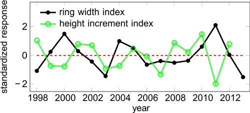
Fig. 1. Standardized response variables i.e. indices for ring width (RWI) and height increment (HII).
We computed the intercorrelations of the detrended target variable (bi-weight mean over all other trees), and each individual tree (Figure S3, available as a supplementary file). Most of the individual trees were highly correlated with the master chronology. There were 6 outliers out of 28 trees with respect to ring widths; with respect to height growth, only the smallest tree was an outlier. The expressed population signals using R package dplR were 0.74 and 0.52 for detrended ring widths and height increments, respectively. Even though we had relatively few trees, especially for height growth, the analysed trees showed reasonably consistent signals.
2.4 Data analysis methods
2.4.1 Fixed time analysis with one to four predictors
As a starting point, we computed linear correlations between each independent variable before and during the growth period and each target variable. We used linear models in order to restrict the search space and reduce the risk of overfitting (Hastie et al. 2001), i.e., a situation where a model is so flexible that it fits the sample data to every detail, but fails to capture the essential features of the unseen data. The correlations were statistically significant (two tailed t-test) at 5% level of significance if the absolute correlation with the radial increment indices was higher than 0.49, and with the height increment indices higher than 0.51. The goal of this analysis was to get a basic understanding about the relationships at a single variable level, while further modelling analysed the combinations of variables.
For the second objective, we built and analysed regression models on one, two, three or four independent variables to predict the annual variation in height and cambial growth. The models are referred to as greedy fixed-time models, because in these models all the independent variables come from equal time intervals. First, we generated all possible models using the standard linear regression. There were 465 models with two explanatory variables, 4495 models with three variables, and 31 465 with four variables. Then the models were filtered out based on their testing accuracy score using a pattern mining approach. Testing accuracy score is measured as the coefficient of determination (R2) on data not used in model fitting via cross-validation procedure, described later. The main principle of the pattern mining approach is that for a more complex model to be selected, the testing accuracy for this model has to be better than the accuracy of any of the models built on subsets of its variables. For example, a model built on A, B, C must be better than models built on A and B, B and C, A and C, and models built only on A, only on B, and only on C.
One-variable fixed-time models were the simplest models build with only one explanatory variable. A separate model was built for each environmental variable in Table 1. The time of year, which had the maximum absolute correlation with the response variable, was selected.
Traditional fixed-time models included two explanatory variables, which are often used in modelling tree growth (e.g. Garcia-Suarez et al. 2009): air temperature and precipitation. The times of year for each variable were chosen such that they had the maximum absolute correlation alone with the response variables.
For each model, we report two performance measures: R2 fit and R2 test. R2 fit is the traditional coefficient of determination, measured on the data used for model fitting. It gives information about the goodness of the model fit. For the baseline predictor that always predicts a constant value, R2 fit = 0. R2 can be negative, which means that the performance is worse than the baseline. R2 test is a coefficient of determination, computed in the same way, but the predictions are made on data that has not been used for model fitting. We used the leave-one-out cross-validation procedure (LOOCV), see e.g. Hastie et al. (2001) for more details. Firstly, parameter estimation was done on all observations except one. Then, a prediction was made for the remaining observation. The procedure was repeated as many times as there were observations in the dataset. For example, ring width observations were available for the years 1998–2013. First we selected the year 1998 as a test-year. Models were fitted on the years 1999–2013 and tested on 1998. Next, the year 1999 was a test year. Models were fitted on the years 1998, 2000–2013, and tested on 1999, etc.
Before each model fitting, we standardized the explanatory variables to zero-mean and unit-variance. When LOOCV procedure was used, the parameters for standardization were computed on the training data while no parameter fitting was done on the testing data. Missing values were replaced by the mean. When LOOCV procedure was used, means were estimated on only training data. The response variables were converted back to the original representation (growth indices) before computing R2 measures.
We also report a consistency index, which indicates how consistent the best time of year is during LOOCV. It was computed as the number of observations for which the most frequent time of year appeared, divided by the total number of observations. Consistency, 1 means that at each iteration of the cross validation cycle the same four-week period is nominated as the most informative. If the value is close to 0, then the time selection is very inconsistent.
2.4.2 Variable time analysis with different number of predictors
Least Angle Regression (LARS, Efron et al. 2004) is a regression technique designed for high dimensional data. It iteratively adds predictors to the regression model taking into account dependencies between predictors. The result is a linear model, but the procedure of parameter fitting results to different coefficients from the standard linear regression. We selected LARS technique to analyse how the number of variables affects the model accuracy, i.e. to what extent high number of partly intercorrelated explanatory variables result in tangled models with low accuracy, and whether the results can be improved by the expert-based pre-selection of candidate variables.
We used the R package ‘lars’ implementation where the maximum number of variables was set to 10 and analysed the occurrence of the parameter values (from 1 to 10). Models obtained by LARS did not have any time constraints. Explanatory variables from any time of year (43 time windows) could have been included, also containing several time periods for an explanatory variable. We used LARS technique for fitting the regression models with three approaches in variable selection:
1: BB, black-box had no restrictions on candidate variables, the selection pool was 31 × 43 = 1333 variables (Table 1),
2: MS, manual pre-selection of 13 variables that have occurred in earlier studies (indicated in Table 1), the selection pool was 13 × 43 = 559 variables, and
3: TR, traditional pre-selection, where only two variables: air temperature and precipitation were allowed, but they could come from any time of year, the selection pool was 2 × 43 = 86 variables.
The analysis was based on the variable selection while fitting LARS regression via cross-validation. For each iteration of LOOCV, a regression model was built. For each variable, we took an average over all the regression coefficients from all LOOCV models. We scaled each coefficient by the total number of candidate variables considered. This way the magnitude of the regression coefficients produced by all three types of any-time models (BB, TS and TR) became comparable. The higher the absolute magnitude of the coefficient, the more important the variable is when considered in a set together with all other variables.
In addition to LARS models, we considered a Baseline model, which does not use any explanatory variables, but always predicts a constant value, equal to the mean of the target variable.
We made the dataset as well as the code implementing our experiments in R publicly available (https://github.com/zliobaite/tree-growth-smear).
3 Results
3.1 Fixed time models
3.1.1 Correlation analysis
There were several periods when individual variables showed consistent correlations with RWI for three or more pixels (i.e. ≥8 weeks, Fig. 2):
1. During the supposed growing season, relative humidity and water vapour were negatively correlated with RWI. Air temperature, carbon gain (GPP), PAR and precipitation during the growing period did not strongly correlate with RWI.
2. Just before or in the early phase of the supposed growing season, air and organic soil temperature, GPP and water vapour concentration positively correlated with RWI while the correlations with global radiation and UVA were negative.
3. Snow depth in the previous winter positively correlated with RWI.
4. Correlations with soil water turned from positive to negative during previous summer
5. GPP in May–Sep in the previous summer (y-1) negatively correlated with RWI while the correlation with NEE was positive for the same period.
6. Soil and air temperatures, water vapour, evapotranspiration and all carbon fluxes (NEE, TER, GPP) negatively correlated with RWI in Jan–Feb in the winter in the previous year (y-1), while the correlation with RH was positive for the same period.
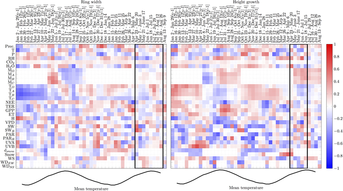
Likewise, several periods were consistently correlated with HII (Fig. 2):
1. During the supposed growing season, RH, soil water and global radiation positively correlated with HII while the correlations with air and soil temperatures and VPD were mostly negative during the same period.
2. Just before or in the early phase of the supposed growing season, RH and snow presence positively correlated with HII while air temperature, TER, GPP, VPD and PAR, UVA and UVB showed negative correlations.
3. Air and soil temperatures and water vapour concentration during winter positively correlated with HII while snow depth, PAR and global radiation showed negative correlations.
4. Precipitation, soil water, RH, GPP, TER and evapotranspiration in the previous summer (y-1) correlated positively with HII, while correlations with VPD, UVA and air temperatures were negative.
5. UVA and UVB in previous spring (y-1) correlated positively with HII while correlation with snow was negative.
6. Soil and air temperatures, water vapour concentration, evapotranspiration and all carbon fluxes (NEE, TER, GPP) in Jan–Feb in the winter in the previous year (y-1) positively correlated with HII while the correlations with snow depth in Jan–Apr (y-1) and radiation in Jan–Mar (y-1) were negative.
3.1.2 One-variable models
The overall predictive power of individual explanatory variables was low for RWI and HII (Table 2ab). Even though R2 was notable in many cases, the testing mostly resulted in negative R2 values indicating that the performance was worse than the baseline. However, for both growth variables, there were a few single predictors individually producing positive R2 test values with high stability. For RWI, those predictors were precipitation during the preceding Dec (y-1), as well as NEE and GPP in April. The predictors producing positive test values for HII were both from preceding year (y-1): UVB during April and NEE in August.
| Table 2a. Predictive accuracies of explanatory variables for the ring width indices. Cons. indicates the consistency index for the best time, R2 fit the coefficient of determination of the model fit on all data and R2 test the coefficient of determination of leave-one-out cross-validation testing. The abbreviations are introduced in Table 1. | ||||
| Feature | Best time | Cons. | R2 fit | R2 test |
| Prec. | Dec 4 – Dec 31 [y-1] | 1 | 0.44 | 0.35 |
| T | Jan 2 – Jan 29 [y-1] | 0.9 | 0.37 | –0.17 |
| P | Dec 4 – Dec 31 [y-1] | 0.9 | 0.3 | –0.91 |
| RH | May 22 – Jun 18 [y-1] | 0.4 | 0.22 | –2.23 |
| CO2 | Aug 13 – Sep 9 | 0.8 | 0.02 | –0.62 |
| H2O | Aug 14 – Sep 10 [y-1] | 0.8 | 0.3 | –0.48 |
| MO | Jul 3 – Jul 30 [y-1] | 0.8 | 0.14 | –0.73 |
| MA | May 22 – Jun 18 [y-1] | 0.8 | 0.12 | –0.56 |
| MB | May 22 – Jun 18 [y-1] | 0.9 | 0.23 | –0.13 |
| MC | May 22 – Jun 18 [y-1] | 0.9 | 0.26 | –0.04 |
| TO | Jul 2 – Jul 29 | 0.3 | 0.17 | –1.28 |
| TA | Jan 16 – Feb 12 [y-1] | 0.9 | 0.34 | –0.68 |
| TB | Jan 16 – Feb 12 [y-1] | 0.9 | 0.43 | –0.07 |
| TC | Jan 2 – Jan 29 [y-1] | 0.8 | 0.3 | –0.37 |
| NEE | Apr 9 – May 6 | 1 | 0.38 | 0.2 |
| TER | Aug 13 – Sep 9 | 0.6 | 0.25 | –0.98 |
| GPP | Apr 9 – May 6 | 1 | 0.42 | 0.26 |
| ET | Jan 2 – Jan 29 [y-1] | 0.6 | 0.12 | –1.45 |
| H | Jan 2 – Jan 29 [y-1] | 0.9 | 0.39 | –0.06 |
| VPD | May 22 – Jun 18 [y-1] | 0.4 | 0.16 | –1.23 |
| SW | Nov 20 – Dec 17 [y-1] | 0.6 | 0.3 | –1.33 |
| SWR | Apr 23 – May 20 | 1 | 0.4 | 0 |
| PAR | May 22 – Jun 18 [y-1] | 0.8 | 0.22 | –0.66 |
| PARR | Aug 28 – Sep 24 [y-1] | 0.8 | 0.26 | –0.96 |
| UVA | Nov 20 – Dec 17 [y-1] | 0.7 | 0.28 | –0.93 |
| UVB | Nov 20 – Dec 17 [y-1] | 0.4 | 0.26 | –1.31 |
| dsnow | Apr 24 – May 21 [y-1] | 0.8 | 0.24 | –5.28 |
| Snow | Apr 24 – May 21 [y-1] | 0.7 | 0.15 | –3.77 |
| WS | Apr 9 – May 6 | 0.6 | 0.2 | –1.29 |
| WDEW | Jun 5 – Jul 2 [y-1] | 0.9 | 0.18 | –1.74 |
| WDNS | Sep 25 – Oct 22 [y-1] | 0.9 | 0.09 | –1.22 |
| Table 2b. Predictive accuracies of explanatory variables for height growth indices. Columns as in Table 2a. | ||||
| Feature | Best time | Cons. | R2 fit | R2 test |
| Prec. | Jan 16 – Feb 12 [y-1] | 0.8 | 0.25 | –1.24 |
| T | Jul 3 – Jul 30 [y-1] | 0.4 | 0.26 | –2.19 |
| P | Feb 12 – Mar 11 | 0.4 | 0.32 | –0.66 |
| RH | Jun 4 – Jul 1 | 0.9 | 0.36 | –0.84 |
| CO2 | Aug 13 – Sep 9 | 0.5 | 0.01 | –0.92 |
| H2O | Apr 23 – May 20 | 0.9 | 0.3 | –0.82 |
| MO | Jun 4 – Jul 1 | 0.6 | 0.14 | –1.19 |
| MA | Jun 4 – Jul 1 | 0.3 | 0.12 | –1.32 |
| MB | May 8 – Jun 4 [y-1] | 0.4 | 0.17 | –1.15 |
| MC | May 22 – Jun 18 [y-1] | 0.8 | 0.13 | –1.2 |
| TO | Jan 16 – Feb 12 [y-1] | 0.9 | 0.29 | –0.84 |
| TA | Jan 2 – Jan 29 [y-1] | 0.8 | 0.25 | –1.21 |
| TB | Jan 2 – Jan 29 [y-1] | 0.9 | 0.22 | –0.62 |
| TC | Nov 20 – Dec 17 [y-1] | 0.3 | 0.08 | –1.2 |
| NEE | Jul 31 – Aug 27 [y-1] | 0.9 | 0.42 | 0.14 |
| TER | Mar 26 – Apr 22 | 0.6 | 0.29 | –0.83 |
| GPP | Jul 31 – Aug 27 [y–1] | 0.9 | 0.38 | –0.27 |
| ET | Jun 18 – Jul 15 | 0.8 | 0.22 | –0.71 |
| H | Jan 2 – Jan 29 [y-1] | 0.8 | 0.34 | –0.76 |
| VPD | Jun 4 – Jul 1 | 0.7 | 0.4 | –0.78 |
| SW | Jul 31 – Aug 27 [y-1] | 0.7 | 0.31 | –0.78 |
| SWR | Sep 25 – Oct 22 [y-1] | 0.6 | 0.31 | –1.59 |
| PAR | Jul 3 – Jul 30 [y-1] | 0.9 | 0.39 | –0.14 |
| PARR | Nov 20 – Dec 17 [y-1] | 0.9 | 0.46 | –0.09 |
| UVA | Jan 29 – Feb 25 | 0.9 | 0.43 | –0.79 |
| UVB | Apr 10 – May 7 [y-1] | 1 | 0.51 | 0.31 |
| dsnow | Nov 6 – Dec 3 [y-1] | 0.4 | 0.17 | –5.13 |
| Snow | Apr 9 – May 6 | 0.9 | 0.38 | –0.6 |
| WS | Mar 12 – Arp 8 | 0.6 | 0.21 | –1.02 |
| WDEW | Sep 25 – Oct 22 [y-1] | 0.8 | 0.29 | –0.2 |
| WDNS | Jun 19 – Jul 16 [y-1] | 0.9 | 0.28 | –0.34 |
3.1.3 Traditional combination of temperature and precipitation
The model for RWI with the two traditionally used explanatory variables (precipitation and air temperature) fitted reasonable well (R2 fit = 0.62) and the generalization was decent (R2 test = 0.27) when periods were as in Table 2a, i.e. precipitation in previous December and air temperature in January (y-1). However, the generalization performance was worse than it would be using only precipitation as a single variable (Table 2a). For HII, the best periods for precipitation and air temperature were in winter and summer in the previous year (Table 2b), respectively. As these were combined, the model fit was low (R2 fit = 0.38) and it failed at generalization i.e. R2 test was lower than the baseline.
3.1.4 Greedy models with 2–4 predictors
Explanatory factors in the RWI models by the greedy approach were mostly related to water (precipitation, soil water, water vapour, evapotranspiration), soil temperature and CO2 uptake (GPP) (Table 3). For HII, explanatory factors related to radiation (PAR, UVB), but also to water (soil water, water vapour, precipitation, snow depth) and CO2 exchange (GPP, NEE), appeared several times (Table 3). The used time periods for the variables were the same as indicated in Table 2ab. For few combinations, the resulting R2 fit and test values were reasonably high in comparison with the models with a single predictor.
| Table 3. Predictive accuracy of selected models with 1–4 predictors for the ring width and height growth indices by the greedy approach. The abbreviations are introduced in Table 1. The used periods are as in Table 2 a and b. | ||||||
| Predictor | R2 fit | R2 test | ||||
| 1 | 2 | 3 | 4 | |||
| Ring width | Prec. | MC | GPP | H | 0.81 | 0.52 |
| H2O | MC | TB | NEE | 0.92 | 0.48 | |
| Prec. | TB | TC | ET | 0.70 | 0.41 | |
| T | MB | MC | SWR | 0.75 | 0.38 | |
| H2O | H | SWR | - | 0.67 | 0.36 | |
| Prec. | NEE | - | - | 0.59 | 0.35 | |
| H2O | MB | TC | GPP | 0.28 | 0.84 | |
| MO | TB | SWR | - | 0.17 | 0.57 | |
| Height growth | PARR | UVB | dsnow | Snow | 0.81 | 0.63 |
| MA | GPP | H | UVB | 0.89 | 0.60 | |
| H2O | TB | NEE | PAR | 0.74 | 0.46 | |
| Prec. | RH | TER | UVB | 0.84 | 0.38 | |
| PAR | UVB | - | - | 0.63 | 0.33 | |
| H2O | GPP | SWR | PARR | 0.77 | 0.31 | |
| MB | TA | NEE | H | 0.17 | 0.79 | |
| NEE | PARR | WD | - | 0.15 | 0.64 | |
3.2 Variable time models
The fit and the test accuracies for Black-Box (BB), manual selection (MS), and traditional (TR) models are reported in Fig. 3. Many test results for the ring width modelling were negative, but TR models with 2–4 selected variables (i.e. periods) performed reasonably well (Fig. 3). The height growth models had a fair fitting performance, but the generalization was generally poor, except for BB approach with one selected variable producing a positive R2 test. The variable was UVB during proceeding April–May (y-1), which also performed well in one-variable models (Table 2b). Generally, the models with fewer input variables did not perform any better than the models with all available input.
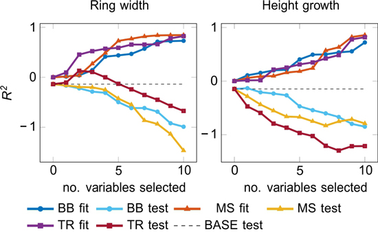
Fig. 3. Accuracy of fit and test models by LARS (see 2.4.2) as a function of the number of included variables.
LARS analysis focused on predictors that appear most often and most consistently in terms of their relation with the target variables. The Black-box model (BB) and the manual selection model (MS) showed similar relations between RWI and weather events (Fig. 4). The remarkable common negative relations were with GPP in the early phase of a growing period, with global radiation during the growing period and snow depth in the previous spring (y-1). Common positive relations rose with global radiation in previous spring. Both models showed mixed relations with precipitation in winter. In addition, BB model indicated negative relation with water vapour concentration in the previous summer (y-1) and UVA in the winter, positive ones with UVA in the spring and reflected radiation during the growth. On the other hand, only MS indicated negative relations with RH in summer and positive ones in winter. The traditional model (TR) with two variables showed mainly positive relation with precipitation in the winter and negative with air temperature in early spring but during the actual growing period all relations were very weak.
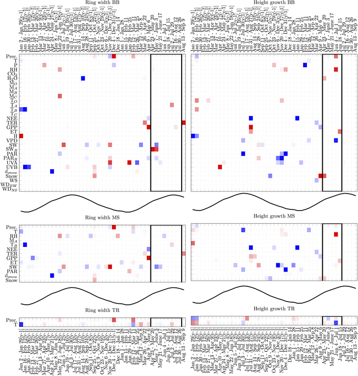
Fig. 4. Analysis of variable selection by LARS in three types of any-time models with different number of candidate predictors (BB, MS and TR). The vertical axis lists variables and the horizontal axis times of year. Black-lined rectangles indicate the most probable actual growing period (Schiestl-Aalto et al. 2015). For time reference, the mean temperature over time is plotted in the middle of the models. Each square is an average over 15–16 models obtained using leave-one-out cross-validation procedure. Blue squares indicate negative relations, and red squares indicate positive relations. Darker colours encode more stable (consistent) performance over multiple trials. Abbreviations are introduced in Table 1. View larger in new window/tab.
BB and MS models showed some similar relations between HII and weather events as well (Fig. 4). The common positive relations were with RH during growth and GPP during previous summer. Common negative relations were NEE during previous summer and early year, and PAR in previous winter and summer. In addition, BB showed negative relations with reflected PAR in winter, air pressure in late winter and VPD during the growing period. Positive relations only by BB were UVB in previous spring (y-1) and snow presence in the early phase of growing season. On the other hand, only MS showed negative relations with temperature during previous summer and global radiation in the winter. The relations between HII and air temperature during previous summer and during the timing of actual growth were negative with TR model.
4 Discussion
4.1 Performance of data-driven models
We investigated which environmental variables sampled at which time periods of the years had the strongest relation to the annual radial and height increment indices. The task setting was non-trivial because there were only a small number of observations of the dependent variables (15–16) for the time when SMEAR data was available, while there were a large number of independent variables from different time periods within the study years. Selected greedy models with fixed time periods demonstrated the best performance whereas several single variables gave positive R2 test values, but their overall performance was not up to scale to predict annual growth variation.
Since annual tree growth is a complex process, consisting of cumulative responses to several simultaneous and fluctuating internal and external factors, it is challenging to model the annual growth variation using a temporally averaged period in a single or in a few environmental factors. This approach may yield more consistent results if longer time series were available, but even the exploration over 16 years is an interesting step forward, as this is the first time when so wide a variety of measurements at so high a resolution have been related to tree growth using data mining techniques.
Modelling using the traditional combination of air temperature and precipitation was not sufficient to predict the tree growth since the used periods, selected only by the correlation analysis, may be not the most effective ones for growth. Combining one to four of any single variables on their best times resulted in better test performances but most of the combinations were not consistent with respect to earlier findings and knowledge of the growth process. The Black Box models were clearly too flexible and resulted in overfitting i.e. they achieved in a good model fit but the generalization performance was poor. Even the decrease in the number of variables did not increase the predictive accuracy. The introduced models may have captured some essential factors, but they would require more evaluation and iterative validation to achieve credibility for example as a mixture of data-driven and first principle modeling approaches. Removing the effects of known affecting factors by traditional methods and mining the residuals, for example, could be one step forward.
Nevertheless, the visual examination of the consistent correlations (Fig. 2) over the high-frequency dataset provided new insights even when the build models were not very powerful. The analysis revealed numerous and, in some cases, lagged correlations with both height and diameter growth of trees. Some of the correlations likely result from the short time series in combination with high dimensional dataset, but there also seems to be a consistent pattern in them. Height and diameter growth correlated partially to different factors with very different delays and often respond in an opposite manner to the same factors.
4.2 Height increment
The buds of Scots pine are formed in July–August, whereas the actual elongation takes place in the following year. Therefore, the conditions during the bud formation are influential for the height increment (Salminen and Jalkanen 2007; Schiestl-Aalto et al. 2013). The consistent correlations found in this study suggest that high GPP together with high soil water content and low water demand for transpiration (high RH, low VPD, and low air temperature) during the bud forming period are favourable for height increment during the following summer. High water content in air and soil maintains tree water potential and turgor pressure needed in forming new cells (Pantin et al. 2012). GPP on the other hand promotes material for new cells but also for turgor maintenance (Pantin et al. 2012).
Against earlier findings from Northern latitudes (Salminen and Jalkanen 2007), this study indicated a negative correlation between air temperature during the bud forming period and height increment. This could indicate that high temperature increases transpirational demand which reduces the water potential of the tree and also may decrease the net carbon uptake and the capability to invest in buds. In addition, a decrease in soil water potential may lead apart from low shoot turgor pressure, also to decreased shoot:root ratio (Brunner et al. 2016), causing a competing sink for the assimilates.
During the period when the actual growth takes place, circumstances supporting the high water potential of the tree (soil moisture, RH, precipitation, water vapour concentration) are beneficial for the height increment, whereas circumstances lowering the water potential (high air temperature and VPD) effect negatively. Also the positive correlations with springtime RH and negative correlations with radiation, VPD and air temperature indicate that circumstances accompanied with low transpirational demand favouring high turgor pressure in the early spring are beneficial for the height growth.
UVB radiation in the preceding spring (y-1) unexpectedly showed a strong positive correlation with the height increment in all analyses. Ren et al. (2006) studied Populus species and found that UVB radiation significantly decreased height growth. High UVB may point to high radiation in general that in combination with low temperatures are harmful for needles in spring (Öquist and Huner 2003; Ensminger et al. 2004; Porcar-Castell et al. 2008) and thus, cause growth losses to be compensated in the following year.
The individual correlations and coefficients, such as the positive correlations or coefficients between the height increment and temperatures, water vapour concentration, evapotranspiration and carbon fluxes accompanied with negative correlations with snow and radiation during the dormant period more than one year earlier (y-1) are difficult to explain. They could result from the whole tree level structural changes reflecting changes in allocation or alterations, e.g., in hormonal control or some other, unknown reason. It cannot be ruled out that some of the correlations are due to coincidences in a relatively short time series. The low overall predictive power of individual explanatory variables and the models by the greedy approach indicates that not all found correlations are meaningful. For example, the sensible heat flux that is roughly the incoming radiation minus evapotranspiration appears as predictor in the regression models for height and diameter growth. The sensible heat flux depends on radiation, moisture conditions, biological activity etc. hardly having by its own a causal relation to growth.
4.3 Ring width
There were no consistent correlations between the meteorological conditions and ring width during the supposed cambial growth period. Only air humidity and atmospheric water vapour concentration showed slightly negative correlations and VPD slightly positive correlation to ring width indicating, that unlike with height growth, diameter growth was favoured by dry weather during the growing period. This could reflect the fact that growth at the lower part of a stem is not critically limited by air humidity conditions and the level of water potential, which is always higher at the lower part of a stem than at shoots (Zimmermann 1983). Also this combination of conditions is normally favourable for photosynthetic production (Chan et al. 2015).
Summer temperature often correlates with ring width (Mäkinen et al. 2001; Korpela et al. 2011; Grudd 2008; Seo et al. 2011), but our results do not support this indicating again that air temperature during the growing period does not limit the growth in the studied site. Our results are, however, similar with those of Hordo et al. (2011) who found that the temperature in current year March–April correlated positively with Scots pine radial growth in southern Finland and Estonia. Warm spring may also favour the recovery of xylem and phloem transport capacity after winter (Vanhatalo et al. 2015) and for certain extend the growing season that reflects as larger accumulated growth at certain fixed time points.
Our analyses also indicate that high GPP at the beginning of the growing season promotes radial growth supporting the findings of Schiestl-Aalto et al. (2015), Chan et al. (2015) and Babst et al. (2014). The role of early carbon gain can be seen also in the negative correlation with NEE, whose negative values indicate carbon uptake as opposed to GPP. In the spring, high GPP may act as a trigger for the onset of cell division or give compensation for the off-season respiratory losses and thus positively affect tree carbon balance. Alternatively, high GPP in the early spring may indicate earlier onset for the growing season. Rossi et al. (2006) suggested that in cold environments, conifers synchronize the maximum growth rate of tree-ring formation with day length. If the growth were culminated by day length, the early onset would simply increase the annual ring width. On the other hand, Chan et al. (2015) showed that a large amount of recently photosynthesized carbon increased daily growth in spring, so perhaps GPP in the early season stands out in the correlations since sugars have an important role both as a growth resource for cell differentiation and as a factor behind sufficient cell turgor together with water availability.
5 Conclusion
The models produced by the data-driven approaches lacked predictive power to firmly identify strong drivers for growth variation at our study site in southern Finland. The accuracy of the prediction did not increase even if the number of candidate explanatory variables was manually decreased in the massive dataset. However, the approach highlighted several interesting aspects on the annual variation in the height and diameter growth of Scots pine: the growth of the Scots pine trees was not promoted by high temperatures during the growing or bud forming periods. Instead, height growth was favoured by a weather that supported high water potential and carbon gain during the bud forming period, and by circumstances maintaining high water potential during the elongation period. A winter with high precipitation and a long-lasting snow cover and a spring with high photosynthetic production indicated promoted diameter growth during the oncoming summer.
Acknowledgements
This study was supported by the Academy of Finland (257641, 277623) and the Academy of Finland Finnish Centre of Excellence Program (272041). We thank Janne Levula for the increment core measurements.
References
Ågren G.I. (1996). Nitrogen productivity or photosynthesis minus respiration to calculate plant growth? Oikos 76(3): 529–535. http://dx.doi.org/10.2307/3546346.
Aloni R. (2013). Role of hormones in controlling vascular differentiation and the mechanism of lateral root initiation. Planta 238(5): 819–830. http://dx.doi.org/10.1007/s00425-013-1927-8.
Babst F., Bouriaud O., Papale D., Gielen B., Janssens I.A., Nikinmaa E., Ibrom A., Wu J., Bernhofer C., Koestner B., Gruenwald T., Seufert G., Ciais P., Frank D. (2014). Above-ground woody carbon sequestration measured from tree rings is coherent with net ecosystem productivity at five eddy-covariance sites. New Phytologist 201(4): 1289–1303. http://dx.doi.org/10.1111/nph.12589.
Babst F., Carrer M., Poulter B., Urbinati C., Neuwirth B., Frank D. (2012). 500 years of regional forest growth variability and links to climatic extreme events in Europe. Environmental Research Letters 7: 045705. http://dx.doi.org/10.1088/1748-9326/7/4/045705.
Bäck J., Aalto J., Henriksson M., Hakola H., He Q., Boy M. (2012). Chemodiversity of a Scots pine stand and implications for terpene air concentrations. Biogeosciences 9(2): 689–702. http://dx.doi.org/10.5194/bg-9-689-2012.
Berninger F., Hari P., Nikinmaa E., Lindholm M., Meriläinen J. (2004). Use of modeled photosynthesis and decomposition to describe tree growth at the northern tree line. Tree Physiology 24(2): 193–204. http://dx.doi.org/10.1093/treephys/24.2.193.
Briffa K.R., Schweingruber F.H., Jones P.D., Osborn T.J., Shiyatov S.G., Vaganov E.A. (1998). Reduced sensitivity of recent tree-growth to temperature at high northern latitudes. Nature 391: 678–682. http://dx.doi.org/10.1038/35596.
Brunner I., Herzog C., Dawes M.A., Arend M., Sperisen C. (2015). How tree roots respond to drought. Frontiers in Plant Science 6(547): 1–16. http://dx.doi.org/10.3389/fpls.2015.00547.
Bunn A.G. (2008). A dendrochronology program library in R (dplR). Dendrochronologia 26(2): 115–124. http://dx.doi.org/10.1016/j.dendro.2008.01.002.
Cajander A.K. (1926). The theory of forest types. Acta Forestalia Fennica 29. 108 p.
Chan T., Höltta T., Berninger F., Mäkinen H., Nöjd P., Mencuccini M., Nikinmaa E. (2016). Separating water-potential induced swelling and shrinking from measured radial stem variations reveals a cambial growth and osmotic concentration signal. Plant Cell and Environment 39(2): 233–244. http://dx.doi.org/10.1111/pce.12541.
Cook E. (1985). A time series analysis approach to tree ring standardization. PhD thesis, University of Arizona.
Cook E.R., Kairiūkštis L.A. (1990). Methods of dendrochronology: applications in the environmental sciences. Springer. ISBN 13: 978-0792305866.
D’Arrigo R., Kaufmann R., Davi N., Jacoby G., Laskowski C., Myneni R., Cherubini P. (2004). Thresholds for warming-induced growth decline at elevational tree line in the Yukon Territory, Canada. Global Biogeochemical Cycles 18, GB3021. 7 p. http://dx.doi.org/10.1029/2004GB002249.
De Schepper V., Steppe K. (2010). Development and verification of a water and sugar transport model using measured stem diameter variations. Journal of Experimental Botany 61(8): 2083–2099. http://dx.doi.org/10.1093/jxb/erq018.
Efron B., Hastie T., Johnstone I., Tibshirani R. (2004). Least angle regression. Annals of Statistics 32(2): 407–451. http://dx.doi.org/10.1214/009053604000000067.
Ensminger I., Sveshnikov D., Campbell D.A., Funk C., Jansson S., Lloyd J., Shibistova O., Öquist G. (2004). Intermittent low temperatures constrain spring recovery of photosynthesis in boreal Scots pine forests. Global Change Biology 10(6): 995–1008. http://dx.doi.org/10.1111/j.1365-2486.2004.00781.x.
Garcia-Suarez A.M., Butler C.J., Baillie M.G.L. (2009). Climate signal in tree-ring chronologies in a temperate climate: a multi-species approach. Dendrochronologia 27(3): 183–198. http://dx.doi.org/10.1016/j.dendro.2009.05.003.
Gea-Izquierdo G., Bergeron Y., Huang J., Lapointe-Garant M., Grace J., Berninger F. (2014). The relationship between productivity and tree-ring growth in boreal coniferous forests. Boreal Environment Research 19: 363–378.
Gough C.M., Vogel C.S., Schmid H.P., Su H.-B, Curtis P.S. (2008). Multi-year convergence of biometric and meteorological estimates of forest carbon storage. Agricultural and Forest Meteorology 148(2): 158–170. http://dx.doi.org/10.1016/j.agrformet.2007.08.004.
Grudd H. (2008). Torneträsk tree-ring width and density AD 500–2004: a test of climatic sensitivity and a new 1500-year reconstruction of north Fennoscandian summers. Climate Dynamics 31(7): 843–857. http://dx.doi.org/10.1007/s00382-007-0358-2.
Hari P., Kulmala M. (2005). Station for measuring ecosystem-atmosphere relations (SMEAR II). Boreal Environment Research 10: 315–322.
Hari P., Sirén G. (1972). Influence of some ecological factors and the seasonal stage of development upon the annual ring width and radial growth index. Royal College of Forestry Department of Reforestation Stockholm Research Notes. 40. 22 p.
Hari P., Havimo M., Koupaei K.K., Jögiste K., Kangur A., Salkinoja-Salonen M., Aakala T., Aalto J., Schiestl-Aalto P., Liski J., Nikinmaa E. (2013) Dynamics of carbon and nitrogen fluxes and pools in forest ecosystem. In: Hari P., Heliövaara K., Kulmala L. (eds). Physical and physiological forest ecology. Springer, Netherlands. p 349–396.
Hastie T., Tibshirani R., Friedman J. (2001). The elements of statistical learning. Springer Series in Statistics, Springer. 533 p.
Helama S., Mielikäinen K., Timonen M., Herva H., Tuomenvirta H., Venäläinen A. (2013). Regional climatic signals in Scots pine growth with insights into snow and soil associations. Dendrobiology 70: 27–34. http://dx.doi.org/10.12657/denbio.070.003.
Henttonen H.M., Mäkinen H., Heiskanen J., Peltoniemi M., Laurén A., Hordo M. (2014). Response of radial increment variation of Scots pine to temperature, precipitation and soil water content along a latitudinal gradient across Finland and Estonia. Agricultural and Forest Meteorology 198–199: 294–308. http://dx.doi.org/10.1016/j.agrformet.2014.09.004.
Höltta T., Mäkinen H., Nöjd P., Mäkelä A., Nikinmaa E. (2010). A physiological model of softwood cambial growth. Tree Physiology 30(10): 1235–1252. http://dx.doi.org/10.1093/treephys/tpq068.
Hordo M., Henttonen H.M., Mäkinen H., Helama S., Kiviste A. (2011). Annual growth variation of Scots pine in Estonia and Finland. Baltic Forestry 17: 35–49.
Ilvesniemi H., Pumpanen J., Duursma R., Hari P., Keronen P., Kolari P., Kulmala M., Mammarella I., Nikinmaa E., Rannik Ü., Pohja T., Siivola E., Vesala T. (2010). Water balance of a boreal Scots pine forest. Boreal Environment Research 15: 375–396.
Kolari P., Kulmala L., Pumpanen J., Launiainen S., Ilvesniemi H., Hari P., Nikinmaa E. (2009). CO2 exchange and component CO2 fluxes of a boreal Scots pine forest. Boreal Environment Research 14: 761–783.
Körner C. (2003). Carbon limitation in trees. Journal of Ecology 91(1): 4–17. http://dx.doi.org/10.1046/j.1365-2745.2003.00742.x.
Korpela M., Nöjd P., Hollmén J., Mäkinen H., Sulkava M., Hari P. (2011). Photosynthesis, temperature and radial growth of Scots pine in northern Finland: identifying the influential time intervals. Trees-Structure and Function 25(2): 323–332. http://dx.doi.org/10.1007/s00468-010-0508-8.
Launiainen S., Rinne J., Pumpanen J., Kulmala L., Kolari P., Keronen P., Siivola E., Pohja T., Hari P., Vesala T. (2005). Eddy covariance measurements of CO2 and sensible and latent heat fluxes during a full year in a boreal pine forest trunk-space. Boreal Environment Research 10: 569–588.
Lanner R.M. (1976). Patterns of shoot development in Pinus and their relationship to growth potential. In: Cannell M.G.R., Last F.T. (eds.). Tree physiology and yield improvement. Academic Press, London, UK. p. 223–243.
Li G., Harrison S.P., Prentice I.C., Falster D. (2014). Simulation of tree-ring widths with a model for primary production, carbon allocation, and growth. Biogeosciences 11(23): 6711–6724. http://dx.doi.org/10.5194/bg-11-6711-2014.
Mäkelä A., Berninger F., Hari P. (1996). Optimal control of gas exchange during drought: theoretical analysis. Annals of Botany 77(5): 461–467. http://dx.doi.org/10.1006/anbo.1996.0056.
Mäkinen H., Nöjd P., Mielikäinen K. (2001). Climatic signal in annual growth variation in damaged and healthy stands of Norway spruce [Picea abies (L.) Karst.] in southern Finland. Trees-Structure and Function 15(3): 177–185. http://dx.doi.org/10.1007/s004680100089.
Mammarella I., Launiainen S., Grönholm T., Keronen P., Pumpanen J., Rannik Ü., Vesala T. (2009). Relative humidity effect on the high-frequency attenuation of water vapor flux measured by a closed-path Eddy covariance system. Journal of Atmospheric and Oceanic Technology 26: 1856–1866. http://dx.doi.org/10.1175/2009JTECHA1179.1.
Millard P., Sommerkorn M., Grelet G. (2007). Environmental change and carbon limitation in trees: a biochemical, ecophysiological and ecosystem appraisal. New Phytologist 175(1): 11–28. http://dx.doi.org/10.1111/j.1469-8137.2007.02079.x.
Misson L. (2004). MAIDEN: a model for analyzing ecosystem processes in dendroecology. Canadian Journal of Forest Research-Revue Canadienne De Recherche Forestiere 34(4): 874–887. http://dx.doi.org/10.1139/X03-252.
Ohtsuka T., Saigusa N., Koizumi H. (2009). On linking multiyear biometric measurements of tree growth with eddy covariance-based net ecosystem production. Global Change Biology 15(4): 1015–1024. http://dx.doi.org/10.1111/j.1365-2486.2008.01800.x.
Olesen J.E., Carter T.R., Diaz-Ambrona C.H., Fronzek S., Heidmann T., Hickler T., Holt T., Minguez M.I., Morales P., Palutikof J.P., Quemada M., Ruiz-Ramos M., Rubaek G.H., Sau F., Smith B., Sykes M.T. (2007). Uncertainties in projected impacts of climate change on European agriculture and terrestrial ecosystems based on scenarios from regional climate models. Climatic Change 81(1): 123–143. http://dx.doi.org/10.1007/s10584-006-9216-1.
Öquist G., Huner N.P.A. (2003). Photosynthesis of overwintering evergreen plants. Annual Review of Plant Biology 54: 329–355. http://dx.doi.org/10.1146/annurev.arplant.54.072402.115741.
Pantin F., Simonneau T., Muller B. (2012). Coming of leaf age: control of growth by hydraulics and metabolics during leaf ontogeny. New Phytologist 196(2): 349–366. http://dx.doi.org/10.1111/j.1469-8137.2012.04273.x.
Parry J.L. (1985). Mathematical-modeling and computer-simulation of heat and mass-transfer in agricultural grain drying – a review. Journal of Agricultural Engineering Research 32(1): 1–29. http://dx.doi.org/10.1016/0021-8634(85)90116-7.
Pichler P., Oberhuber W. (2007). Radial growth response of coniferous forest trees in an inner Alpine environment to heat-wave in 2003. Forest Ecology and Management 242(2–3): 688–699. http://dx.doi.org/10.1016/j.foreco.2007.02.007.
Pirinen P., Simola H., Aalto J., Kaukoranta J.-P., Karlsson P., Ruuhela R. (2012). Tilastoja Suomen ilmastosta 1981–2010 - Climatological statistics of Finland 1981–2010. 83 p.
Porcar-Castell A., Juurola E., Ensminger I., Berninger F., Hari P., Nikinmaa E. (2008). Seasonal acclimation of photosystem II in Pinus sylvestris. II. Using the rate constants of sustained thermal energy dissipation and photochemistry to study the effect of the light environment. Tree Physiology 28(10): 1483–1491. http://dx.doi.org/10.1093/treephys/28.10.1483.
Ren J., Yao Y.N., Yang Y.Q., Korpelainen H., Junttila O., Li C.Y. (2006). Growth and physiological responses to supplemental UV-B radiation of two contrasting poplar species. Tree Physiology 26(5): 665–672. http://dx.doi.org/10.1093/treephys/26.5.665.
Rocha A.V., Goulden M.L., Dunn A.L., Wofsy S.C. (2006). On linking interannual tree ring variability with observations of whole-forest CO2 flux. Global Change Biology 12(8): 1378–1389. http://dx.doi.org/10.1111/j.1365-2486.2006.01179.x.
Rossi S., Deslauriers A., Anfodillo T., Morin H., Saracino A., Motta R., Borghetti M. (2006). Conifers in cold environments synchronize maximum growth rate of tree-ring formation with day length. New Phytologist 170(2): 301–310. http://dx.doi.org/10.1111/j.1469-8137.2006.01660.x.
Sala A., Woodruff D.R., Meinzer F.C. (2012). Carbon dynamics in trees: feast or famine? Tree Physiology 32(6): 764–775. http://dx.doi.org/10.1093/treephys/tpr143.
Salminen H., Jalkanen R. (2007). Intra-annual height increment of Pinus sylvestris at high latitudes in Finland. Tree Physiology 27(9): 1347–1353. http://dx.doi.org/10.1093/treephys/27.9.1347.
Schiestl-Aalto P., Nikinmaa E., Mäkelä A. (2013). Duration of shoot elongation in Scots pine varies within the crown and between years. Annals of Botany 112(6): 1181–1191. http://dx.doi.org/10.1093/aob/mct180.
Schiestl-Aalto P., Kulmala L., Mäkinen H., Nikinmaa E., Mäkelä A. (2015). CASSIA – a dynamic model for predicting intra-annual sink demand and interannual growth variation in Scots pine. New Phytologist 206(2): 647–659. http://dx.doi.org/10.1111/nph.13275.
Seo J., Eckstein D., Jalkanen R., Schmitt U. (2011). Climatic control of intra- and inter-annual wood-formation dynamics of Scots pine in northern Finland. Environmental and Experimental Botany 72(3): 422–431. http://dx.doi.org/10.1016/j.envexpbot.2011.01.003.
Vaganov E.A., Hughes M.K., Kirdyanov A.V., Schweingruber F.H., Silkin P.P. (1999). Influence of snowfall and melt timing on tree growth in subarctic Eurasia. Nature 400: 149–151. http://dx.doi.org/10.1038/22087.
Vanhatalo A., Chan T., Aalto J., Korhonen J.F., Kolari P., Höltta T., Nikinmaa E., Bäck J. (2015). Tree water relations can trigger monoterpene emissions from Scots pine stems during spring recovery. Biogeosciences 12: 5353–5363. http://dx.doi.org/10.5194/bg-12-5353-2015.
Vesala T., Haataja J., Aalto P., Altimir N., Buzorius G., Garam E., Hämeri K., Ilvesniemi H., Jokinen V., Keronen P., Lahti T., Markkanen T., Mäkelä J.M., Nikinmaa E., Palmroth S., Palva L., Pohja T., Pumpanen J., Rannik Ü., Siivola E., Ylitalo H., Hari P., Kulmala M. (1998). Long-term field measurements of atmosphere-surface interactions in boreal forest combining forest ecology, micrometeorology, aerosol physics and atmospheric chemistry. Trends in Heat, Mass & Momentum Transfer 4: 17–35.
Vesala T., Suni T., Rannik U., Keronen P., Markkanen T., Sevanto S., Grönholm T., Smolander S., Kulmala M., Ilvesniemi H., Ojansuu R., Uotila A., Levula J., Mäkelä A., Pumpanen J., Kolari P., Kulmala L., Altimir N., Berninger F., Nikinmaa E., Hari P. (2005). Effect of thinning on surface fluxes in a boreal forest. Global Biogeochemical Cycles 19, GB2001. http://dx.doi.org/10.1029/2004GB002316.
Xu B., Yang Y., Li P., Shen H., Fang J. (2014). Global patterns of ecosystem carbon flux in forests: a biometric data-based synthesis. Global Biogeochemical Cycles 28(9): 962–973. http://dx.doi.org/10.1002/2013GB004593.
Zimmermann M.H. (1983) Xylem structure and the ascent of sap. Springer-Verlag, Berlin.
Zubizarreta-Gerendiain A., Gort-Oromi J., Mehtätalo L., Peltola H., Venäläinen A., Pulkkinen P. (2012). Effects of cambial age, clone and climatic factors on ring width and ring density in Norway spruce (Picea abies) in southeastern Finland. Forest Ecology and Management 263: 9–16. http://dx.doi.org/10.1016/j.foreco.2011.09.011.
Zweifel R., Zimmermann L., Zeugin F., Newbery D.M. (2006). Intra-annual radial growth and water relations of trees: implications towards a growth mechanism. Journal of Experimental Botany 57(6): 1445–1459. http://dx.doi.org/10.1093/jxb/erj125.
Zweifel R., Eugster W., Etzold S., Dobbertin M., Buchmann N., Haesler R. (2010). Link between continuous stem radius changes and net ecosystem productivity of a subalpine Norway spruce forest in the Swiss Alps. New Phytologist 187(3): 819–830. http://dx.doi.org/10.1111/j.1469-8137.2010.03301.x.
Total of 66 references.
