Karol Przeździecki  ,
Jarosław Zawadzki,
Chris Cieszewski,
Pete Bettinger
,
Jarosław Zawadzki,
Chris Cieszewski,
Pete Bettinger
Estimation of soil moisture across broad landscapes of Georgia and South Carolina using the triangle method applied to MODIS satellite imagery
Przeździecki K., Zawadzki J., Cieszewski C., Bettinger P. (2017). Estimation of soil moisture across broad landscapes of Georgia and South Carolina using the triangle method applied to MODIS satellite imagery. Silva Fennica vol. 51 no. 4 article id 1683. https://doi.org/10.14214/sf.1683
Highlights
- Temperature vegetation dryness indices were calculated from MODIS satellite imagery to estimate subsurface soil moisture at different depths using the triangle method
- Observations were carried out over the vast areas of Georgia and South Carolina, USA, covered with diverse land uses that, included dense forests and agricultural areas
- The triangle method may be useful in forestry management applications where the productivity potential of a region and the hydrologic role of forests in that region are of concern.
Abstract
We describe here a study based on analysis of vegetation indices and land surface temperatures, which provides relevant information for estimating soil moisture at regional scales. Through an analysis of MODIS satellite imagery and in situ moisture data, the triangle method was used to develop a conceptual land surface temperature−vegetation index model, and spatial temperature-vegetation dryness index (TVDI) values to describe soil moisture relationships for a broad landscape. This study was situated mainly within two states of the southern United States (Georgia and South Carolina). The total study area was about 30 million hectares. The analyses were conducted using information gathered from the 2009 growing season (from the end of March to September). The results of the study showed that soil moisture content was inversely proportional to TVDI, and that TVDI based on the normalized difference vegetation index (NDVI) had a slightly higher correlation with soil moisture than TVDI based on the enhanced vegetation index (EVI).
Keywords
soil moisture;
remotely sensed imagery;
satellite observations of forests;
triangle method;
TVDI;
MODIS
-
Przeździecki,
Warsaw University of Technology, Faculty of Building Services, Hydro and Environmental Engineering, 00-653, Nowowiejska 20, Warszawa, Poland
 http://orcid.org/0000-0002-2275-5223
E-mail
karol_przezdziecki@is.pw.edu.pl
http://orcid.org/0000-0002-2275-5223
E-mail
karol_przezdziecki@is.pw.edu.pl
-
Zawadzki,
Warsaw University of Technology, Faculty of Building Services, Hydro and Environmental Engineering, 00-653, Nowowiejska 20, Warszawa, Poland
http://orcid.org/0000-0003-2842-0018
E-mail
j.j.zawadzki@gmail.com
-
Cieszewski,
University of Georgia, Warnell School of Forestry and Natural Resources, 180 E Green St, Athens, GA 30602, USA
http://orcid.org/0000-0003-2842-4406
E-mail
thebiomat@gmail.com
-
Bettinger,
University of Georgia, Warnell School of Forestry and Natural Resources, 180 E Green St, Athens, GA 30602, USA
http://orcid.org/0000-0002-5454-3970
E-mail
pbettinger@warnell.uga.edu
Received 9 August 2016 Accepted 10 July 2017 Published 21 July 2017
Views 168724
Available at https://doi.org/10.14214/sf.1683 | Download PDF

1 Introduction
Soil moisture serves as a vital factor supporting ecosystem service, and has a direct influence on vegetation growth and nutrient cycling. Its assessment plays an important role in efforts to monitor and analyze the environment (Oschner et al. 2013). Soil moisture is often considered along with soil nutrients and composition as a key factor in determining ecosystem productivity and site quality, forming the basis for site quality and productivity classifications. More recently, scientists have discussed the importance of soil moisture as a factor in climate change and broad-scale hydrologic cycles (Chen et al. 2011b). Land surface parameters, such as soil moisture, temperature, and land cover are important components of ecosystem processes on both local and global scales (Meng et al. 2009; Nelson et al. 2011; Kim et al. 2012; Lowe and Cieszewski 2014). The complexity of the soil environment, the diversity of land cover (particularly vegetation cover), and the impact of other factors such as terrain and topography, make soil moisture research especially challenging and very expensive to perform in the field (Byun et al. 2014; de Tomás et al. 2014). For these reasons there is an increasing interest within the scientific community in development of methods for soil moisture and water availability assessment using remotely sensed imagery (Lowe et al. 2009; Petropoulos et al. 2015). The increasing availability of remotely sensed imagery, coupled with advances in availability of computing technology, contributes to advances in cost-efficient broad-scale monitoring of environmental phenomena (Łukowski and Usowicz 2014). Satellite technology also facilitates timely and cost effective assessments of vegetation, through indices such as the normalized difference vegetation index (NDVI) (Rouse et al. 1974), which have been widely used for assessment of drought conditions (Kogan 1995; Ji and Peters 2003; Bajgiran et al. 2008; Jain et al. 2009; Karnieli et al. 2010).
The primary advantage of basing analyses on vegetation indices is that over a short time frame they are not very sensitive to corresponding changes in soil moisture, because the presence of chlorophyll in vegetation does not change immediately at the onset of water stress. When water stress begins in trees, leaves remain green for some time and change only after a prolonged stressful period. On the contrary, land surface temperature is strongly affected by both soil moisture content and the vegetation canopy (or lack of thereof). Vegetation shading and vegetation transpiration are representative of evaporation processes and affect the moisture content of soils. In forest management areas, regional soil moisture conditions may be correlated with regional annual tree growth and site productivity. This relationship can influence the outcomes of fiber supply assessments and associated forecasts, and supply-demand-price prediction studies. These forest management and planning issues have important associations with the sustainability of forests, while analyses of soil moisture and vegetation indices can improve our understanding of the hydrologic role of forests (Cho et al. 2016). If one wanted to stratify the forests based on potential site quality (Cieszewski et al. 2005; Iles 2009), soil moisture, forest age, and vegetation indices, these processes may facilitate an understanding of broad-scale productivity, growth potential, and hazards (fire and forest health). It may also then be possible to observe specific hydrologic phenomena such as spatial diversification in water conditions caused by depression cones around coal mines (Miatkowski et al. 2013).
To facilitate the development of broad-scale soil moisture estimates, remotely sensed Moderate Resolution Imaging Spectroradiometer (MODIS) data have been used (Wan et al. 2004; Li et al. 2008; Mallick et al. 2009; Patel et al. 2009; Rhee et al. 2010; Son et al. 2012) to estimate temperature-vegetation dryness index (TVDI), which can be derived from land surface temperature (LST), normalized difference vegetation index (NDVI) and enhanced vegetation index (EVI) values. A number of earlier studies (Wang et al. 2004; Wan et al. 2004; Sun et al. 2008; Li et al. 2008; Mallick et al. 2009; Wang et al. 2010; Chen et al. 2011a; Liu et al. 2016) have also advocated the use of TVDI for monitoring surface moisture conditions. TDVI has been recently applied to studies of forests in Brazil (Cho et al. 2016), Argentina (Holzman et al. 2014), and China (Chen et al. 2015). The primary advantage of this approach is that TVDI combines the information captured by both vegetation indices and LST, which facilitates wider application of assessments of soil moisture conditions across diverse landscapes.
The theoretical range of TVDI values is 0to 1; larger TVDI values define drier conditions, and smaller TVDI values defined wetter conditions. In order to estimate soil moisture content in a given specific area, TVDI values need to be calibrated to the local conditions based on local data, correlating TVDI values with measurements of soil moisture conditions recorded in the area of interest. The use of these types of models in association with local calibration is in some way similar to the use of the site index models in forest management and biometrics. In essence, general models are developed based on large sets of relevant regional data, and then the general models are subsequently localized to specific conditions based on small samples of local site measurements.
In this study, we describe a method for estimating soil moisture that is based on analysis of vegetation indices (NDVI and EVI) and LST. The analytical process is called the triangle method, introduced by Sandholt et al. (2002). The basic idea of the triangle method is that the surface temperatures and vegetation indices are correlated with soil moisture and vegetation cover density, which can be assessed through appropriate analysis. Sandholt et al. (2002) present the theoretical background for the estimation of TVDI, which is based on a scatter plot of remotely sensed vegetation index and land surface temperatures. In a simplified approach, the scatter plot should form a triangle (Fig. 1), in which areas close to the upper edge in the scatter plot represent drier land conditions than those close to the lower edge. In theory, the wet edge of the conceptual model should form a horizontal line, where land surface or forest canopy temperature is independent of the vegetation index. There are no water stress conditions present along this line where the soil moisture and evapotranspiration capacity are relatively high (Chen et al. 2015). However, the wet edge could also have a positive or negative slope depending on the relationship between the vegetation index and the surface temperature assumptions for the landscape and season under study, and where data may be lacking for certain landscape conditions (Sandholt et al. 2002; Cho et al. 2016). Areas near the dry edge represent stressed conditions of limited water availability for plants, and minimal evaporation (when the vegetation index decreases) or minimal transpiration in case of dense vegetation canopy (where the vegetation index is close to 1). Scatter plots are often trapezoidal as well (Chen et al. 2015), where the triangle becomes truncated with larger vegetation index values. Through the triangle method, TVDI values for a landscape are derived. TVDI has been successfully applied in monitoring, and subsequent assessments, of regional droughts (Yang et al. 2008; Liu et al. 2016), and it can be effective in soil moisture status for different types of land uses (Chen et al. 2015). The triangle method has been applied to a variety of landscapes, such as western Africa (Sandholt et al. 2002), the central region of Spain (de Tomás et al. 2014), and northern China (Yang et al. 2008).
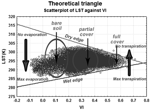
Fig. 1. Land surface temperature (LST) values plotted against a vegetation index (VI), forming a theoretical triangle model.
The objective of this study is to apply the triangle method of soil moisture assessment to an important timber-producing area of the world, using MODIS satellite imagery. The triangle method can be relevant to forest management planning efforts, and to growth and yield predictions, due to its relationship to water availability, which plays the most vital role in measuring forest productivity. In essence, assessments of soil moisture across broad areas of important timber-producing regions can inform society about growth and yield potential of that region; and therefore, it may improve our understanding of the hydrologic role of forests (Chen et al. 2015; Cho et al. 2016). Thus, this research addresses a relevant issue of concern for forestry and for management of forest ecosystems, and can help increase our understanding of forest ecosystems, their productivities, and the sustainable use and conservation of forest resources.
2 Material and methods
2.1 Study area
The study area encompassed mainly the states of Georgia and South Carolina in the southeastern United States (Fig. 2), while some portions of other neighboring states were also included in the analysis. This area is situated between 30°18´N to 35°15´N latitude and 78°30´W to 85°30´W longitude. The lengths of the east-west and north-south edges of the study area were approximately 730 km and 500 km, respectively. The majority of the study area has a humid subtropical climate, with mild winter and hot, humid summer seasons. Annual precipitation in this region varies from 1000 mm to 2000 mm. Most of the forest land (over 80 percent) in both Georgia and South Carolina is owned by private landowners (individuals, forest industry, and other corporate owners).
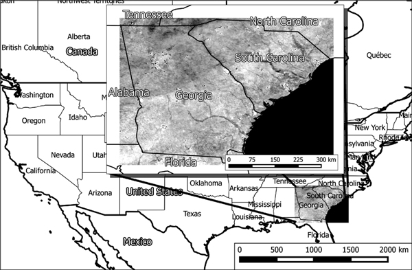
Fig. 2. The study area, located in the southeastern United States.
Georgia contains about 15.4 million hectares (ha) of land, of which 10.0 million ha are forested in areas that range from the southern edge of the Appalachian Mountains to the Coastal Plain along the Atlantic Ocean. Loblolly pine (Pinus taeda L.) and slash pine (Pinus elliottii Engelm.) are the most pervasive conifers. Sweetgum (Liquidambar styraciflua L.), yellow-poplar (Liriodendron tulipifera L.), white oak (Quercus alba L.), water oak (Quercus nigra L.), swamp tupelo (Nyssa sylvatica Marshall), and red maple (Acer rubrum L.) are the most pervasive deciduous tree species (Brandeis and Hartsell 2016). Other lands in Georgia consist mainly of agricultural and developed areas. South Carolina contains about 8.3 million ha of land, of which 5.3 million ha are forest lands. As with Georgia, the landforms in South Carolina range from the southern end of the Appalachian Mountains to the Coastal Plain, and other lands consist mainly of agricultural and developed areas. With the exception of slash pine, the types of forests found in South Carolina are very similar to the types of forests in Georgia (Brandeis et al. 2016). In both states, the amount of forested area has remained relatively stable in recent years, but there is continual flux (both gains and losses) between forests and agriculture and developed uses. This region has had some severe droughts in the recent past; one drought period between 2004 and 2007 resulted in a severe water crisis (Missimer et al. 2014).
2.2 Satellite imagery
A MODIS sensor is installed on two spacecrafts (Terra and Aqua) operated by the U.S. National Aeronautical and Space Administration (NASA) (U.S. Geological Survey 2014). In our work, we used only the MODIS data collected from the Terra spacecraft, which operates on sun-synchronous orbit with an equatorial overpass time of 10:30. The MODIS sensor has a viewing swath width of 2330 km and a temporal resolution of one to two days. Two types of MODIS data products were used in this study: MOD13A2 (Vegetation Index Product) and MOD11A2 (Land Surface Temperature Product). MOD13A2 is a 16-day composite of vegetation indices; MOD11A2 is 8-day composite of land surface temperature and emissivity. Both of these data products have spatial resolution of 1 km. Prior to acquisition, the data products underwent atmospheric corrections for gases, aerosol scattering, and thin cirrus clouds. They both are considered to have passed through the third level of processing (level-3) in version 005 of the data. From the MOD11A2 science data sets, we used the LST_Day_1km layer, and a quality assurance layer (QC_day). MOD11A2 products have better than 1 Kelvin degree accuracy (0.5 K in most cases) (National Aeronautics and Space Administration 2009). The quality assurance layer provides information that allows one to exclude from consideration certain pixels of unacceptable quality. From the MOD13A2 data, we used the 16 days NDVI and the 16 days EVI layers and a quality assurance layer (1_km_16 days_VI_Quality). A more complete description of these can be found in Solano et al. (2010). Our analyses considered eleven 16-day periods from 22 March 2009 to 13 September 2009 (Table 1).
| Table 1. Beginning and ending times of data collection by MODIS satellite during each of the eleven 16-day periods considered in this study. | ||
| Period | Beginning date (time 00:00:00) | Ending date (time 23:59:59) |
| 1 | 22-Mar-2009 | 6-April-2009 |
| 2 | 7-April-2009 | 22-April-2009 |
| 3 | 23-April-2009 | 8-May-2009 |
| 4 | 9-May-2009 | 24-May-2009 |
| 5 | 25-May-2009 | 9-June-2009 |
| 6 | 10-June-2009 | 25-June-2009 |
| 7 | 26-June-2009 | 11-July-2009 |
| 8 | 12-July-2009 | 27-July-2009 |
| 9 | 28-July-2009 | 12-August-2009 |
| 10 | 13-August-2009 | 28-August-2009 |
| 11 | 29-August-2009 | 13-September-2009 |
2.3 In situ soil moisture data
Measurements of soil moisture were acquired from the International Soil Moisture Network (Dorigo et al. 2011a; Dorigo et al. 2011b), an international cooperative for development and maintenance of the global in situ soil moisture database. This database is an essential tool for the geoscientific community for calibrating and improving global satellite observations and land surface models. Station locations (Fig. 3) are representative of the climate of the region, and are not heavily influenced by unique local factors or microclimates (National Oceanic and Atmospheric Administration 2015). The analyzed data (Table 2) were collected by five stations belonging to the Soil Climate Analysis Network (SCAN) and two stations belonging to the U.S. Climate Reference Network (USCRN). However, one station from the USCRN only provided soil moisture data from September 13, 2009 forward, so in this case it contributed only to the 5 last time periods of our analysis, from periods 7 to 11 (Table 1). While the USCRN had two other measurement stations that were located within our study area, these stations did not collect soil moisture measurements during our period of study. A statistical summary of in situ data is presented in Table 3. While ground measurements from the International Soil Moisture Network were available at several soil depths, we only selected the first three soils depths (5 cm, 10 cm, and 20 cm) for our analysis. These had closer correspondence with the on-ground vegetation more reliably captured by the satellite imagery.
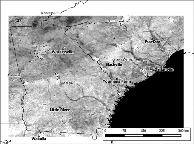
Fig. 3. Locations and names of the in situ moisture measurement stations in the study area.
| Table 2. Names of in situ moisture measurement stations, their networks, and geographic coordinates, for the analyzed data. | ||||
| Station number | Station name | Latitude, Longitude | Network | Vegetation type a |
| 1 | Little River | 31°30´N, 83°30´W | SCAN | Agriculture |
| 2 | Pee Dee | 34°18´N, 79°44´W | SCAN | Agriculture, young pine plantation, old deciduous forest |
| 3 | Wakulla | 30°18´N, 84°25´W | SCAN | Middle-aged pine plantation |
| 4 | Watkinsville | 33°53´N, 83°26´W | SCAN | Agriculture, developed areas |
| 5 | Youmans Farm | 32°40´N, 81°12´W | SCAN | Agriculture, old pine forest |
| 6 | Blackville | 33°21´N, 81°20´W | USCRN | Agriculture |
| 7 | McClellanville | 33°09´N, 79°22´W | USCRN | Agriculture, deciduous forest |
| a Vegetation types in the immediate area (100 m) around each measurement point. | ||||
| Table 3. Statistical summary of the in situ moisture data used for parameterization into moisture units (m3 m–3). | ||||||||
| Soil depth | Parameter | Little River | Pee Dee | Wakulla | Watkinsville | Youmans Farm | Blackville | McClellanville |
| cm | - | m3 m–3 | m3 m–3 | m3 m–3 | m3 m–3 | m3 m–3 | m3 m–3 | m3 m–3 |
| 5 | Minimum | 0.037 | 0.063 | 0.014 | 0.111 | 0.027 | 0.034 | 0.022 |
| Maximum | 0.338 | 0.296 | 0.140 | 0.405 | 0.327 | 0.213 | 0.110 | |
| Mean | 0.103 | 0.189 | 0.066 | 0.204 | 0.123 | 0.103 | 0.052 | |
| Std. Dev. | 0.038 | 0.055 | 0.029 | 0.069 | 0.058 | 0.055 | 0.017 | |
| 10 | Minimum | 0.047 | 0.051 | 0.029 | 0.054 | 0.038 | 0.047 | 0.019 |
| Maximum | 0.369 | 0.251 | 0.144 | 0.327 | 0.304 | 0.171 | 0.111 | |
| Mean | 0.102 | 0.162 | 0.077 | 0.121 | 0.142 | 0.089 | 0.063 | |
| Std. Dev. | 0.035 | 0.046 | 0.025 | 0.052 | 0.058 | 0.038 | 0.022 | |
| 20 | Minimum | 0.056 | 0.048 | 0.010 | 0.067 | 0.030 | 0.210 | 0.012 |
| Maximum | 0.229 | 0.209 | 0.103 | 0.331 | 0.288 | 0.290 | 0.133 | |
| Mean | 0.116 | 0.137 | 0.060 | 0.128 | 0.137 | 0.240 | 0.076 | |
| Std. Dev. | 0.036 | 0.039 | 0.022 | 0.054 | 0.061 | 0.025 | 0.028 | |
Choosing the best depth of soil moisture field measurements for validation of satellite observations is not a trivial task. Most of regional observations in optical and infrared bands use subsurface soil moisture measurements of 0to 20 cm (Wang et al. 2007; Zhang et al. 2015; Liu et al. 2016). In case of satellite radiometric measurements, effective penetration depths of C and L type microwaves in soils are commonly in the range of 0–5 cm (Mohanty et al. 2017). At the same time, the greatest availability of soil moisture field measurements, such as gravimetric, TDR (Time Domain Reflectometry) ones, as well as measurements from meteorological stations, come from soil surface or its shallow depths. There also exist some computational techniques, as the exponential filter filter approachone, allowing for calculating soil moisture at greater depths using its surface values (Albergel et al. 2008; Kędzior and Zawadzki 2016).
In this study we used all existing soil moisture data in the public domain available at the time of the study for the study timeframe.
Soil moisture data were obtained using hydraprobe analog sensors (2.5 Volt), which are coaxial impedance dielectric reflectometry sensors. Measurement stations provided the soil moisture data on an hourly basis. However, MODIS data for the research area were acquired only once between 9 and 11 AM UTC time. Therefore, we estimated the value of each soil moisture data point as an average of measurements taken at 9, 10 and 11 AM, UTC time. The estimated soil moisture data from these measurements, taken at these times, were developed for eleven time periods, for each of the seven measurement stations. The total number of measurements considered at the three soil depths was 693 (3 hours × 3 soil depths × 7 stations × 11 time periods). When combined, that should produce 231 periodic (9 AM to 11 AM) averages. However, some data were missing. For example, there were 9 points that did not have ground measurements available, and two points (McClellanville and Blackville) where data were only available for five periods of time. Furthermore, data for one site (Little River) did not have measurements for the 20 cm soil depth during the last 3 periods. There were also 11 points in time associated with each soil depth that did not have valid MODIS pixel values, either due to the presence of clouds or due to other imaging problems. Thus, while a total of 693 observation points were intended for the analysis, in actuality 522 measurements were used, resulting in 174 periodic averages.
2.4 Data processing
Due to differences in temporal resolution, two MOD11A2 composites and one MOD13A2 composite were used in each 16-day period. Namely, two MOD11A2 8-day composites were averaged to match one MOD13A2 16-day composite. Data processing consisted of masking, mosaicking, reprojecting and scaling the remotely sensed imagery, which is a standard in this type of analysis, and it ensures increased level of comparability between the produced results and outcomes of other similar studies. Pixels with poor quality vegetation index, as defined in the MOD13A2 (1_km_16 days_VI_Quality) vegetation index quality specifications were masked out (excluded) from further processing (Land Processes Distributed Active Archive Center 2014). This processing step was performed using the Land Data Operational Product Evaluation (LDOPE) software provided by the MODIS land quality assessment group (Roy et al. 2002). Mosaicking was performed using the MODIS Reprojection Tool (MRT), and the resulting products are HDF-EOS files projected to tile-based sinusoidal projection (Earth Resources Observations and Science Center 2011). The projection was subsequently changed from sinusoidal to Universal Transverse Mercator. Reprojection was based on a nearest neighbor (NN) method, a necessity for resampling without changing layer values, because the mask consisted of two values (1 and 0). Finally, images were rescaled to LST in Kelvin degrees or to vegetation indices values.
2.5 The triangle method
The triangle method is applicable to analysis of broad landscapes, because the land surface temperature vegetation index triangle space emerges only for large areas. This is so because the variability in surface moisture and vegetation cover conditions are too great to be meaningfully visualized across small areas (Sun et al. 2012). The primary challenge in this study was to estimate parameters of equations defining the wet and dry edge conditions within the land surface temperature vegetation index triangle space. This is an important issue because the distance of particular land area (pixel) to a wet or dry edge is illustrative of the soil moisture condition represented by that area on the ground. Pixels close to a wet edge are wetter and those that are close to a dry edge, are comparatively drier. Calculations of wet and dry edge coefficients were developed using linear regression methods.
In order to calculate parameters of the dry and wet edges, the NDVI and EVI were partitioned into small subdomains with an interval of 0.02. From these subdomains we chose the highest value of LST for dry edge and the lowest value of LST for the wet edge. According to Chen et al. (2011b) only pixels with a NDVI value higher than 0.2–0.3 were chosen as calculating dry edge parameters, because dry edge of the triangle has approximately regular shapes in this range. The TVDI can be calculated on the basis of defined edges (Liu et al. 2016; Cho et al. 2016) as:

, where:
LST = the daytime land surface temperature of a pixel
VI = vegetation index value of a pixel (either NDVI or EVI)
LSTmin(VI), LSTmax(VI) = minimum and maximum land surface temperatures for a given vegetation index calculated from functions related to the wet and dry edges:
![]()
![]()
, where:
amax, bmax = estimable regression parameters (intercept and slope) for the dry edge
amin, bmin = estimable regression parameters (intercept and slope) for the wet edge
(a listing of the program in the MATLAB environment for the dry and wet edges calculation is available upon request from K. Przeździecki).
The slopes (bmin, bmax) and intercepts (amin, amax) of the wet and dry edges are the most crucial parameters for the estimation. Parameters of the wet edge describe the condition of soil moisture saturation. Parameters of the dry edge describe the condition where there is no water accessible to vegetation. The in situ ground measurement data are presented as volumetric water contents. We estimated three linear regression models, one for each soil depth, to define the relationships between TVDI and soil moisture. The TVDI estimate for the pixels representing the in situ soil moisture measurement stations were used to develop the regression models:
![]()
, where:
ai, bi = the estimable model parameters for soil depth i
ei = the normally distributed error with mean equal zero for soil depth i
i = a soil depth
MCi = the calibrated local data moisture content (m3 m–3) for soil depth i
TVDI = Temperature-Vegetation Dryness Index, based on either NDVI or EVI
Finally, we calculated the coefficients of determination (R2) for all the three regression models using values from all of the measurement periods. We also established relationships between (a) TVDI(NDVI) and soil moisture, and (b) TVDI(EVI) and soil moisture, on which basis we could compile maps of soil moisture conditions in moisture units (m3 m–3) for the three soil depths.
3 Results
Parameters developed to describe dry edges (LSTmax) and wet edges (LSTmin) (Table 4) of the land surface temperature models suggested that the resulting triangle models for vegetation index / land surface temperature were triangular in shape, but not necessarily right triangular as suggested by the theoretical model. For example, the wet edge slope (bmin) of the triangle models using NDVI as the vegetation index was positive (upward sloping) during measurement periods 1–5 and 8–11. However, during periods 6 and 7 the slope of the wet edge was almost horizontal or negative (downward sloping). When EVI was used as the vegetation index, a similar pattern was observed (Table 4); although, the slope of the wet edge remained positive and was much more upward-sloping during measurement periods 8–11. As expected, the slope of the dry edge (bmax) was negative for both vegetation indices, and was often steeper sloping when NDVI was used than when EVI was used as the vegetation index. The fact that the empirical models are shaped as truncated triangles (Fig. 4), but not necessarily right triangles, is consistent with other published research (Sandholt et al. 2002). The temporal evolution of parameters was similar for both (a) TVDI based on NDVI and (b) TVDI based on EVI, which is consistent with other similar studies in the literature (Yang et al. 2008; Chen et al. 2011b; Zawadzki et al. 2016). However, during periods of reduced soil moisture availability, such as measurement period 6 in Fig. 4, the wet and dry edges have contracted, indicating stressed conditions and limited water availability for plants in much of the studied region.
| Table 4. Parameters for dry and wet edges of the calculated “triangles” for each of the analyzed eleven 16-day periods. | ||||||||
| Period | TVDI(NDVI) | TVDI(EVI) | ||||||
| Wet edge | Dry edge | Wet edge | Dry edge | |||||
| amin | bmin | amax | bmax | amin | bmin | amax | bmax | |
| 1 | 264.0 | 33.0 | 315.2 | –19.2 | 279.0 | 19.1 | 310.0 | –19.0 |
| 2 | 273.0 | 20.5 | 318.0 | –23.0 | 283.1 | 13.8 | 311.2 | –22.5 |
| 3 | 272.8 | 24.6 | 338.0 | –40.0 | 284.0 | 16.3 | 325.0 | –34.0 |
| 4 | 278.0 | 10.0 | 337.2 | –38.0 | 282.0 | 8.0 | 324.8 | –32.0 |
| 5 | 267.0 | 26.0 | 340.6 | –39.0 | 280.6 | 16.0 | 324.0 | –28.0 |
| 6 | 289.8 | 3.0 | 330.8 | –25.5 | 291.4 | 1.9 | 333.0 | –38.0 |
| 7 | 297.0 | –7.4 | 351.2 | –49.0 | 286.2 | 6.0 | 340.0 | –49.0 |
| 8 | 268.2 | 22.6 | 341.2 | –40.0 | 267.4 | 30.8 | 326.0 | –29.5 |
| 9 | 253.8 | 42.0 | 343.0 | –42.5 | 260.0 | 42.0 | 323.4 | –26.8 |
| 10 | 237.0 | 59.0 | 340.0 | –41.0 | 246.0 | 62.0 | 320.0 | –22.4 |
| 11 | 247.0 | 44.0 | 346.0 | –47.0 | 249.1 | 60.5 | 313.0 | –12.0 |
| Average | 268.0 | 25.2 | 336.5 | –36.7 | 273.5 | 25.1 | 322.8 | –28.5 |
| amax, bmax = linear regression parameters for the dry edge amin, bmin = linear regression parameters for the wet edge TVDI – Temperature Vegetation Dryness Index NDVI – Normalized Difference Vegetation Index EVI – Enhanced Vegetation Index | ||||||||
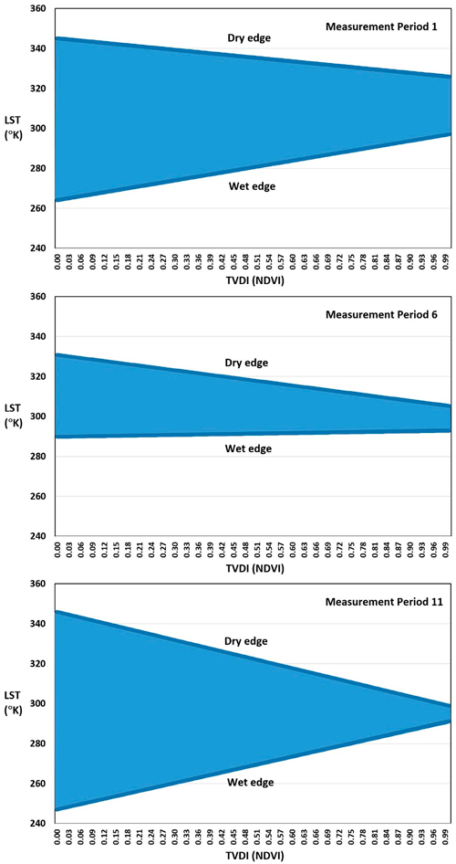
Fig. 4. Triangular relationships developed for the study area through the use of land surface temperature (LST) and Temperature Vegetation Dryness Index (TVDI) based on the Normalized Difference Vegetation Dryness index (NDVI).
As expected, TVDI values in our study increased with decreasing soil moisture (Fig. 5). All of the relationships were linear and had weak to moderate coefficients of determination (R2) for the six TDVI and soil moisture relationships (two vegetation indices, three soil depths). In most cases the correlation between TDVI and soil moisture for the three soil depths varied from weak to moderate and was statistically significant at α = 0.01 level, except for the correlation between soil moisture at the depth of 20 cm and TVDI calculated from EVI, which was statistically significant at α = 0.02. The detailed p-values are given in Fig. 5. Other researchers investigating the parameterization of TVDI values have obtained similar results even with much larger sets of measurement points (Chen et al. 2011b). The results did not reveal any significant discrepancy among the three different soil depths.
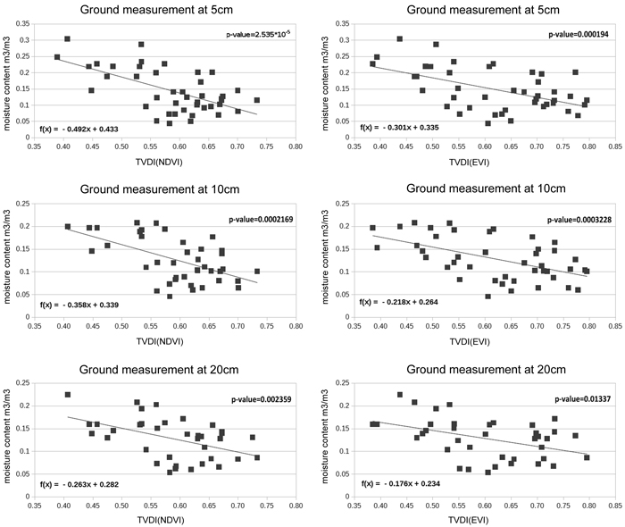
Fig. 5. Scatterplots with regression lines for in situ soil moisture content at three depths a) 5 cm; b) 10 cm; and c) 20 cm predicted from Temperature Vegetation Dryness Index (TVDI) values. P-values for each regression model are also shown. View larger in new window/tab.
Maps produced (Fig. 6) from these analyses illustrate relative values of soil surface moisture across the broad landscape. These estimates are time-dependent, and soil moisture at the three studied depths are correlated, which is expected because the three soils depths are spatially relatively close to each other and there is a fair amount of interaction between them. One can see that the soil moisture levels in Fig. 6 decline with increasing soil depth, suggesting a negative relationship between soil depth and soil moisture level during this measurement period. In addition, from a broad perspective the estimates of soil moisture seem reasonable since areas near major rivers have higher estimated soil moisture than areas further away (upland) and areas containing significant human developments (cities).
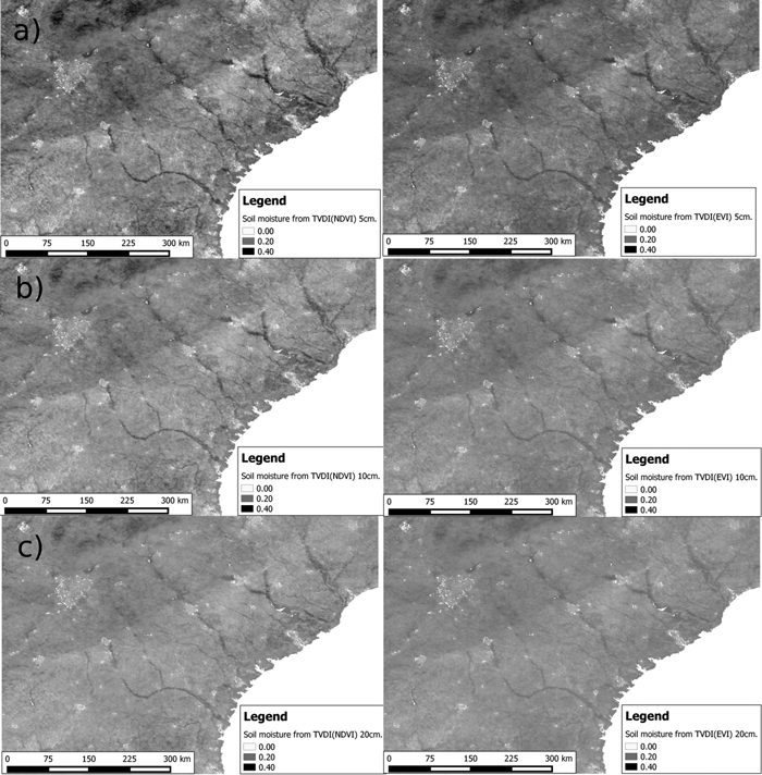
Fig. 6. Map of soil moisture values calculated from the MODIS based on Temperature Vegetation Dryness Index calculated using Normalized Difference Vegetation Index TVDI(NDVI) (left) and Temperature Vegetation Dryness Index calculated using Enhanced Vegetation Dryness Index TVDI(EVI) (right) for three depth measurements during the second study measurement period (April 7–22, 2009): a) 5 cm; b) 10 cm; and c) 20 cm. View larger in new window/tab.
4 Discussion
Vegetation productivity potential can have a major impact on local economies and the standard of living of the people residing in the region. The work we presented here on the triangle method for estimating water conditions may thus be used in various situations where the issues related to vegetation water stress over large areas are relevant. Research on soil moisture estimation using remotely-sensed satellite imagery is very important, both from a scientific point of view as a key factor in modeling processes occurring on the surface of the earth (Wang and Qu 2009), and from an economic point of view given the high correlation of soil moisture to agriculture or forest productivity (Verstraeten et al. 2006). It seems also evident that remote sensing based broad-scale analyses of soil moisture content may offer major financial savings over more time-consuming and costly conventional ground measurements, which would be especially expensive to collect outside of the permanent soil moisture stations currently in operation. There is also the possibility of applying the triangle method to imagery collected with other sensors, such as Landsat 5 Thematic Mapper (prior to its decommissioning), Landsat 7 Enhanced Thematic Mapper + and the more recent Landsat 8 Operational Land Imager and Thermal Infrared Sensor. However, while each of these sensors provide higher spatial resolution than MODIS imagery, for broad areas they pose more complex data management challenge in both: the spatial estimation of soil moisture, and the development of appropriate site-specific TVDI values around each soil measurement station.
As we have shown, the triangle method provides a way of describing the distribution of forested areas by soil moisture content and vegetation indices, and to portray these relationships graphically within a study area. Soil moisture spatial patterns, in general, have a strong temporal stability (Vachaud et al. 1985) even for large areas that range in size from 100 to 1000 km2. Thus the soil moisture temporal pattern observed at one location closely follows the temporal pattern of the spatial average for the given area (Martínez-Fernández and Ceballos 2003; Cosh et al. 2008; Wagner et al. 2008; Brocca et al. 2010), which enabled us to validate the triangle method results using ground soil moisture measurements. Given the resources necessary to monitor soil moisture across a broad region, we were only able to utilize seven measurement stations. Thus one advance would be to have a denser network of spatially distributed measurement stations, from which to collect the data for fitting the models, calibrating them for local conditions, and validating them.
The goodness of fit for the models developed is expressed by the coefficient of determination (R2) of each model fitting, which indicates the proportion of the variance in the dependent variable that was explained, during the model fitting by the independent variable. The relationships between TVDI and soil moisture are weak to moderate, but still reasonable and informative of soil moisture levels under different vegetation or land use conditions. As suggested above, additional resources could increase the accuracy of the model and allow for a more comprehensive validation analysis. The data from permanent soil measurement stations were sparse, but systematic and obtained through a single consistent statistical design. In consequence of the data scarcity, all of the available measurements were used in the development of the predictive models. Any further reduction of the data by reserving some measurements for analytical validation of the soil moisture estimates, without additional significant development of ground measuring network, would have been counterproductive.
Other potential sources of error include: (i) the assumption of a small spatial sample sourced from the individual measurement station locations; (ii) the assumption that satellite data and soil moisture measurement data represent meaningfully the 16-day composite; and (iii) the fact that various vegetation conditions could have slightly different responses to drought conditions. Nevertheless, the presented here results are consistent with the findings of Meng et al. (2008), that the 16-day composites of MODIS data are useful in applications of the triangle method and drought studies. This could be attributed to the fact that the 16-day composites have much better quality than daily MODIS images, and that TVDI, based on vegetation indices, represents an average availability of water accessible to forest plants in the root zone, which is usually much more inertial, and therefore stable, than the surface soil moisture. On the other hand, the impact of two assumptions on the outcomes of the analyses could be evaluated with a more extensive research program, and used to elicit the sensitivity of the models to uncertainties one might assume in the representative data. Further, a more spatially-explicit sensitivity analysis might be designed to examine the impact of fine-scale vegetation conditions on broad-scale soil moisture estimates. These additional studies all seem to be open areas of research today.
5 Conclusions
This research examined the opportunity for using remotely sensed data to estimate soil moisture across broad landscapes. We estimated TVDI using NDVI and EVI that were derived from MODIS satellite imagery and using in situ soil moisture measurements. The analysis was conducted across a broad area from Georgia and South Carolina in the southern United States. Our study found a reasonable relationship between soil moisture content and temperature-vegetation indices. While the triangular relationships did not produce the right triangle models, sometimes associated with the triangle method, they were in agreement with other applied models developed in various parts of the world. The results suggest that vegetation indices derived from remotely sensed imagery may be useful in forest management and planning for assessing current and past soil moisture levels, which may be useful in evaluating potential forest productivity conditions, and may be helpful for assessing the hydrologic condition of the landscape, which is important in all landscape planning, forest management, and conservation endeavors.
Acknowledgements
This work was partly supported by the U.S. Department of Agriculture, National Institute of Food and Agriculture, McIntire-Stennis project 1012166, administered by the University of Georgia, and partly by the Faculty of Building Services, Hydro and Environmental Engineering, Warsaw University of Technology, Poland.
References
Albergel C., Rüdiger C., Pellarin T., Calvet J.-C., Fritz N., Froissard F., Suquia D., Petitpa A., Piguet B., Martin E. (2008). From near-surface to root-zone soil moisture using an exponential filter: an assessment of the method based on in-situ observations and model simulations. Hydrology and Earth Systems Sciences 12(6): 1323–1337. https://doi.org/10.5194/hess-12-1323-2008.
Bajgiran P.R., Darvishsefat A.A., Khalili A., Makhdoum M.F. (2008). Using AVHRR-based vegetation indices for drought monitoring in the Northwest of Iran. Journal of Arid Environments 72(6): 1086–1096. https://doi.org/10.1016/j.jaridenv.2007.12.004.
Brandeis T.J., Hartsell A. (2016). Forests of Georgia, 2014. U.S. Department of Agriculture, Forest Service, Southern Research Station, Asheville, NC. Resource Update FS–72. 4 p.
Brandeis T.J., Hartsell A., Brandeis C., Randolph K., Oswalt S. (2016). Forests of South Carolina, 2015. U.S. Department of Agriculture, Forest Service, Southern Research Station, Asheville, NC. Resource Update FS–102. 4 p.
Brocca L., Melone F., Moramarco T., Wagner W., Hasenauer S. (2010). ASCAT soil wetness index validation through in situ and modeled soil moisture data in central Italy. Remote Sensing of Environment 114(11): 2745–2755. https://doi.org/10.1016/j.rse.2010.06.009.
Byun K., Liaqat U.W., Choi M. (2014). Dual-model approaches for evapotranspiration analyses over homo-and heterogeneous land surface conditions. Agricultural and Forest Meteorology 197: 169–187. https://doi.org/10.1016/j.agrformet.2014.07.001.
Chen C.F., Son N.T., Chang L.Y., Chen C.C. (2011a). Monitoring of soil moisture variability in relation to rice cropping systems in the Vietnamese Mekong Delta using MODIS data. Applied Geography 31(2): 463–475. https://doi.org/10.1016/j.apgeog.2010.10.002.
Chen J., Wang C., Jiang H., Mao L., Yu Z. (2011b). Estimating soil moisture using Temperature–Vegetation Dryness Index (TVDI) in the Huang-huai-hai (HHH) plain. International Journal of Remote Sensing 32(4): 1165−1177. https://doi.org/10.1080/01431160903527421.
Chen S., Wen Z., Jiang H., Zhao Q., Zhang X., Chen Y. (2015). Temperature Vegetation Dryness Index estimation of soil moisture under different tree species. Sustainability 7(9): 11401–11417. https://doi.org/10.3390/su70911401.
Cho J., Ryu J-H., Yeh P.J-F., Lee Y-W., Hong S. (2016). Satellite-based assessment of Amazonian surface dryness due to deforestation. Remote Sensing Letters 7(1): 71–80. https://doi.org/10.1080/2150704X.2015.1109159.
Cieszewski C.J., Iles K., Lowe R.C., Zasada M.J. (2005). Proof of concept for an approach to a finer resolution inventory. In: Proceedings of the fifth annual forest inventory and analysis symposium, McRoberts R.E, Reams G.A, Van Deusen P.C., McWilliams W.H. (eds.). U.S. Department of Agriculture, Forest Service, Washington Office, Washington, D.C. General Technical Report WO-69. p. 69–74.
Cosh M.H., Jackson T.J., Moran S., Bindlish R. (2008). Temporal persistence and stability of surface soil moisture in a semi-arid watershed. Remote Sensing of Environment 112(2): 304−313. https://doi.org/10.1016/j.rse.2007.07.001.
de Tomás A., Nieto H., Guzinski R., Salas J., Sandholt I., Berliner P. (2014). Validation and scale dependencies of the triangle method for the evaporative fraction estimation over heterogeneous areas. Remote Sensing of Environment 152: 493–511. https://doi.org/10.1016/j.rse.2014.06.028.
Dorigo W., van Oevelen P., Wagner W., Drusch M., Mecklenburg S., Robock A., Jackson T. (2011a). A new international network for in-situ soil moisture data. Eos 92(17): 141–142. https://doi.org/10.1029/2011EO170001.
Dorigo W.A., Wagner W., Hohensinn R., Hahn S., Paulik C., Xaver A., Gruber A., Drusch M., Mecklenburg S., van Oevelen P., Robock A., Jackson T. (2011b). The International Soil Moisture Network: a data hosting facility for global in-situ soil moisture measurements. Hydrology and Earth System Sciences 15: 1675–1698. https://doi.org/10.5194/hess-15-1675-2011.
Earth Resources Observations and Science Center (2011). MODIS reprojection tool user’s manual, Release 4.1. U.S. Department of the Interior, U.S. Geological Survey, Earth Resources Observations and Science Center, Sioux Falls, SD.
Holzman M.E., Rivas R., Bayala M. (2014). Subsurface soil moisture estimation by VI-LST method. IEEE Geoscience and Remote Sensing Letters 11(11): 1951–1955. https://doi.org/10.1109/LGRS.2014.2314617.
Iles K. (2009). “Total-Balancing” an inventory: a method for unbiased inventories using highly biased non-sample data at variable scales. Mathematical and Computational Forestry & Natural-Resource Sciences 1(1): 10–13.
Jain S.K., Keshri R., Goswami A., Sarkar A., Chaudhry A. (2009). Identification of drought-vulnerable areas using NOAA AVHRR data. International Journal of Remote Sensing 30(10): 2653–2668. https://doi.org/10.1080/01431160802555788.
Ji L., Peters A.J. (2003). Assessing vegetation response to drought in the northern Great Plains using vegetation and drought indices. Remote Sensing of Environment 87(1): 85–98. https://doi.org/10.1016/S0034-4257(03)00174-3.
Karnieli A., Agam N., Pinker R.T., Anderson M., Imhoff M.L., Gutman G.G., Panov N., Goldberg A. (2010). Use of NDVI and land surface temperature for drought assessment: merits and limitations. Journal of Climate 23(3): 618–633. https://doi.org/10.1175/2009JCLI2900.1.
Kędzior M., Zawadzki J. (2016). Comparative study of soil moisture estimations from SMOS satellite mission, GLDAS database, and cosmic-ray neutrons measurements at COSMOS station in eastern Poland. Geoderma 283: 21–31. https://doi.org/10.1016/j.geoderma.2016.07.023.
Kim H., Bettinger P., Cieszewski C.J. (2012). Reflections on the estimation of stand-level forest characteristics using Landsat satellite imagery. Applied Remote Sensing Journal 2(2): 45–56.
Kogan F.N. (1995). Application of vegetation index and brightness temperature for drought detection. Advances in Space Research 15(11): 91–100. https://doi.org/10.1016/0273-1177(95)00079-T.
Land Processes Distributed Active Archive Center (2014). Vegetation indices 16-day L3 global 1 km. https://lpdaac.usgs.gov/dataset_discovery/modis/modis_products_table/mod13a2. [Cited 20 March 2017].
Li Z., Wang Y., Zhou Q., Wu J., Peng J., Chang H. (2008). Spatiotemporal variability of land surface moisture based on vegetation and temperature characteristics in Northern Shaanxi Loess Plateau, China. Journal of Arid Environments 72(6): 974–985. https://doi.org/10.1016/j.jaridenv.2007.11.014.
Liu H., Zhang A., Jiang T., Lv H., Liu X., Wang H. (2016). The spatiotemporal variation of drought in the Beijing-Tianjin-Hebei Metropolitan Region (BTHMR) based on the modified TVDI. Sustainability 8(12): 1327. https://doi.org/10.3390/su8121327.
Lowe R.C., Cieszewski C.J. (2014). Multi-source K-nearest neighbor, mean balanced forest inventory of Georgia. Mathematical and Computational Forestry & Natural-Resource Sciences 6(2): 65–79.
Lowe R.C., Cieszewski C.J., Liu S., Meng Q., Siry J.P., Zasada M., Zawadzki J. (2009). Assessment of stream management zones and road beautifying buffers in Georgia based on remote sensing and various ground inventory data. Southern Journal of Applied Forestry 33(2):91–100.
Łukowski M., Usowicz B. (2014). Surface soil moisture satellite and ground-based measurements. Acta Agrophysica Monographiae 2014(1). 107 p.
Mallick K., Bhattacharya B.K., Patel N.K. (2009). Estimating volumetric surface moisture content for cropped soils using a soil wetness index based on surface temperature and NDVI. Agricultural and Forest Meteorology 149: 1327–1342. https://doi.org/10.1016/j.agrformet.2009.03.004.
Martínez-Fernández J., Ceballos A. (2003). Temporal stability of soil moisture in a large-field experiment in Spain. Soil Science Society of America Journal 67(6): 1647–1656. https://doi.org/10.2136/sssaj2003.1647.
Meng L., Li J., Chen Z., Xi W., Chen D., Duan H. (2008). The calculation of TVDI based on the composite time of pixel and drought analysis. The International Archives of the Photogrammetry, Remote Sensing and Spatial Information Sciences 38(2): 519–524.
Meng Q., Cieszewski C., Madden M. (2009). Large area forest inventory using Landsat ETM+: A geostatistical approach. ISPRS Journal of Photogrammetry and Remote Sensing 64(1): 27–36. https://doi.org/10.1016/j.isprsjprs.2008.06.006.
Miatkowski Z., Przeździecki K., Zawadzki J. (2013). Observations of spatial diversification of water conditions in permanent grasslands in the visible near infrared spectrum in the impact area of brown coal opencast mine. Annals of Geomatics 11(4): 59–66. [In Polish].
Missimer T.M., Danser P.A., Amy G., Pankratz T. (2014). Water crisis: the metropolitan Atlanta, Georgia , regional water supply conflict. Water Policy 16(4): 669–689. https://doi.org/10.2166/wp.2014.131.
Mohanty B.P., Cosh M.H., Lakshmi V., Montzka C. (2017). Soil moisture remote sensing: state-of-the-science. Vadose Zone Journal 16(1). https://doi.org/10.2136/vzj2016.10.0105.
National Aeronautics and Space Administration (2009). Status for: land surface temperature and emissivity (MOD11). http://landval.gsfc.nasa.gov/ProductStatus.php?ProductID=MOD11. [Cited 25 June 2015].
National Oceanic and Atmospheric Administration (2015). Site selection criteria. http://www.ncdc.noaa.gov/crn/sites.html. [Cited 25 June 2015].
Nelson M.D., Healey S.P., Moser W.K., Masek J.G., Cohen W.B. (2011). Consistency of forest presence and biomass predictions modeled across overlapping spatial and temporal extents. Mathematical and Computational Forestry & Natural-Resource Sciences 3(2): 102–113.
Ochsner T.E., Cosh M.H., Cuenca R.H., Dorigo W.A., Draper C.S., Hagimoto Y., Kerr Y.H., Njoku E.G., Small E.E., Zreda M. (2013). State of the art in large-scale soil moisture monitoring. Soil Science Society of America Journal 7(6):1888–1919. https://doi.org/10.2136/sssaj2013.03.0093.
Patel N.R., Anapashsha R., Kumar S., Saha S.K., Dadhwal V.K. (2009). Assessing potential of MODIS derived temperature/vegetation condition index (TVDI) to infer soil moisture status. International Journal of Remote Sensing 30(1): 23–39. https://doi.org/10.1080/01431160802108497.
Petropoulos G.P., Ireland G., Barrett B. (2015). Surface soil moisture retrievals from remote sensing: current status, products & future trends. Physics and Chemistry of the Earth, Parts A/B/C 83–84: 36–56. https://doi.org/10.1016/j.pce.2015.02.009.
Rhee J., Im J., Carbone G.J. (2010). Monitoring agricultural drought for arid and humid regions using multi-sensor remote sensing data. Remote Sensing of Environment 114(12): 2875–2887. https://doi.org/10.1016/j.rse.2010.07.005.
Rouse J.W. Jr., Hass R.H., Schell J.A., Deering D.W. (1974). Monitoring vegetation systems in the Great Plains with ERTS. In: Freden S.C., Mercanti E.P., Becker M.A. (eds.). The 3rd Earth Resources Technology Satellite-1 symposium. National Aeronautics and Space Administration, Washington, D.C. p. 309–317.
Roy D.P., Borak J.S., Devadiga S., Wolfe R.E., Zheng M., Descloitres J. (2002). The MODIS land product quality assessment approach. Remote Sensing of Environment 83(1–2): 62–76. https://doi.org/10.1016/S0034-4257(02)00087-1.
Sandholt I., Rasmussen K., Andersen J. (2002). A simple interpretation of the surface temperature/vegetation index space for assessment of surface moisture status. Remote Sensing of Environment 79(2–3): 213–224. https://doi.org/10.1016/S0034-4257(01)00274-7.
Solano R., Didan K., Jacobson A., Huete A. (2010). MODIS vegetation indices (MOD13) C5 user’s guide, version 1.00. Terrestrial Biophysics and Remote Sensing Lab, University of Arizona, Tucson, AZ.
Son N.T., Chen C.F., Chen C.R., Chang L.Y., Minh V.Q. (2012). Monitoring agricultural drought in the Lower Mekong Basin using MODIS NDVI and land surface temperature data. International Journal of Applied Earth Observation and Geoinformation 18: 417–427. https://doi.org/10.1016/j.jag.2012.03.014.
Sun L., Sun R., Li X., Liang S., Zhang R. (2012). Monitoring surface soil moisture status based on remotely sensed surface temperature and vegetation index information. Agricultural and Forest Meteorology 166–167: 175–187. https://doi.org/10.1016/j.agrformet.2012.07.015.
Sun W., Wang P.X., Zhang S.Y., Zhu D.H., Liu J.M., Chen J.H., Yang H.S. (2008). Using the vegetation temperature condition index for time series drought occurrence monitoring in the Guanzhong Plain, PR China. International Journal of Remote Sensing 29(17–18): 5133–5144. https://doi.org/10.1080/01431160802036557.
U.S. Geological Survey (2014). MODIS overview. U.S. Department of the Interior, Geological Survey, Reston, VA. https://lpdaac.usgs.gov/dataset_discovery/modis. [Cited 25 June 2015].
Vachaud G., Passerat de Silans A., Balabanis P., Vauclin M. (1985). Temporal stability of spatially measured soil water probability density function. Soil Science Society of America Journal 49(4): 822–828. https://doi.org/10.2136/sssaj1985.03615995004900040006x.
Verstraeten W.W., Veroustraete F., van der Sande C.J., Grootaers I., Feyen J. (2006). Soil moisture retrieval using thermal inertia, determined with visible and thermal spaceborne data, validated for European forests. Remote Sensing of Environment 101(3): 299–314. https://doi.org/10.1016/j.rse.2005.12.016.
Wagner W., Pathe C., Doubkova M., Sabel D., Bartsch A., Hasenauer S., Blöschl G., Scipal K., Martínez-Fernández J., Löw A. (2008). Temporal stability of soil moisture and radar backscatter observed by the Advanced Synthetic Aperture Radar (ASAR). Sensors 8(2): 1174−1197. https://doi.org/10.3390/s80201174.
Wan Z., Wang P., Li X. (2004). Using MODIS land surface temperature and normalized difference vegetation index products for monitoring drought in the southern Great Plains, USA. International Journal of Remote Sensing 25(1) :61–72. https://doi.org/10.1080/0143116031000115328.
Wang C., Qi S., Niu Z., Wang J. (2004). Evaluating soil moisture status in China using he temperature–vegetation dryness index (TVDI). Canadian Journal of Remote Sensing 30(5): 671–679. https://doi.org/10.5589/m04-029.
Wang L., Qu J.J., Zhang S., Hao X.; Dasgupta S. (2007). Soil moisture estimation using MODIS and ground measurements in eastern China. International Journal of Remote Sensing 28(6) 1413–1418. https://doi.org/10.1080/01431160601075525.
Wang H., Li X., Long H., Xu X., Bao Y. (2010). Monitoring the effects of land use and cover type changes on soil moisture using remote-sensing data: a case study in China’s Yongding River basin. Catena 82(3): 135–145. https://doi.org/10.1016/j.catena.2010.05.008.
Wang L., Qu J.J. (2009). Satellite remote sensing applications for surface soil moisture monitoring: a review. Frontiers of Earth Science in China 3(2): 237–247. https://doi.org/10.1007/s11707-009-0023-7.
Yang X., Wu J.J., Shi P.J., Yan F. (2008). Modified triangle method to estimate soil moisture status with MODerate resolution Imaging Spectroradiometer (MODIS) products. The International Archives of Photogrammetry, Remote Sensing and Spatial Information Sciences 37: 555–560.
Zawadzki J., Przeździecki K., Miatkowski Z. (2016). Determining the area of influence of depression cone in the vicinity of lignite mine by means of triangle method and LANDSAT TM/ETM+ satellite images. Journal of Environmental Management 166: 605–614. https://doi.org/10.1016/j.jenvman.2015.11.010.
Zhang J., Zhou Z., Yao F., Yang L., Hao C. (2015). Validating the modified perpendicular drought index in the north China region using in situ soil moisture measurement. IEEE Geoscience Remote Sensing Letters 12(3): 542–546. https://doi.org/10.1109/LGRS.2014.2349957.
Total of 63 references.
