Terje Gobakken,
Lauri Korhonen  ,
Erik Næsset
,
Erik Næsset
Laser-assisted selection of field plots for an area-based forest inventory
Gobakken T., Korhonen L., Næsset E. (2013). Laser-assisted selection of field plots for an area-based forest inventory. Silva Fennica vol. 47 no. 5 article id 943. https://doi.org/10.14214/sf.943
Highlights
- Using laser data as auxiliary information in the selection of field plot locations helps to decrease costs in forest inventories based on airborne laser scanning
- Two independent, differently selected sets of field plots were used for model fitting, and third for validation
- Using partial instead of ordinary least squares had no major influence on the results
- Forty well placed plots produced fairly reliable volume estimates.
Abstract
Field measurements conducted on sample plots are a major cost component in airborne laser scanning (ALS) based forest inventories, as field data is needed to obtain reference variables for the statistical models. The ALS data also provides an excellent source of prior information that may be used in the design phase of the field survey to reduce the size of the field data set. In the current study, we acquired two independent modeling data sets: one with ALS-assisted and another with random plot selection. A third data set was used for validation. One canopy height and one canopy density variable were used as a basis for the ALS-assisted selection. Ordinary and partial least squares regressions for stem volume were fitted for four different strata using the two data sets separately. The results show that the ALS-assisted plot selection helped to decrease the root mean square error (RMSE) of the predicted volume. Although the differences in RMSE were relatively small, models based on random plot selection showed larger mean differences from the reference in the independent validation data. Furthermore, a sub-sampling experiment showed that 40 well placed plots should be enough for fairly reliable predictions.
Keywords
forest inventory;
LIDAR;
airborne laser scanning;
stratified sampling;
area-based approach
- Gobakken, Norwegian University of Life Sciences, Department of Ecology and Natural Resource Management, Ås, Norway E-mail terje.gobakken@umb.no
-
Korhonen,
University of Eastern Finland, School of Forest Sciences, P.O. Box 111, FI-80101 Joensuu, Finland
E-mail
lauri.korhonen@uef.fi
- Næsset, Norwegian University of Life Sciences, Department of Ecology and Natural Resource Management, Ås, Norway E-mail erik.naesset@umb.no
Received 18 June 2013 Accepted 5 November 2013 Published 19 December 2013
Views 123231
Available at https://doi.org/10.14214/sf.943 | Download PDF

1 Introduction
Forest management planning requires reliable stand-level information of the forest resources. This information was traditionally obtained by field surveys, but nowadays remote sensing is commonly used instead, as aerial survey technology has developed rapidly while the costs of field work have increased. Although aerial photography has been used actively in management inventories in many countries since the 1960s, the remote sensing information has mainly been used in manual procedures involving stereo photogrammetry and photo interpretation. With the introduction of airborne laser scanning (ALS) technology it has become possible to utilize the remote sensing information in forest inventories in an automated way. The modern ALS sensors were initially developed for topographical mapping: they emit laser pulses usually at near-infrared wavelengths, and measure distances to terrain below with sub-meter precision based on the flight time of the pulse (Wehr and Lohr 1999). In a forested area, some of the laser pulses reflect from the tree crowns, enabling estimation of canopy height and density (Næsset et al. 2004).
The practical ALS-based inventories are usually conducted using the area-based method (e.g. Næsset 2002; Jensen et al. 2006). A sample of accurately positioned field plots is collected in the inventory area covered by the ALS data. The laser echo locations are intersected with the plot area, allowing the calculation of different metrics related to canopy height and density for each plot. Statistical models are used to relate e.g. field-estimated volume with the ALS metrics, and the models are then applied to obtain wall-to-wall predictions of volume for every forest stand in the whole area. As the method is based on the echo height distribution, the pulse density can be relatively low (< 1 pulse / m2) which decreases the costs. Aerial image variables can also be used as additional predictors in the models (Packalén and Maltamo 2007).
In a statistical sampling context, the area-based inventory method can be characterized as small area estimation using a synthetic estimator (Särndal et al. 1992). The term synthetic estimator indicates that a global model is used to provide local (stand-wise) estimates. Since the stand estimates are obtained as pure predictions provided by a model without any local (stand-wise) correction for bias, the method can also be classified as a pure model-based application. The design of the sample survey is one of the factors that have a major effect on the final outcome of the inventory. In model-based estimation the plot data should cover the entire range of variability (tree species, tree size, site fertility etc.) in the forests of the inventory area, and also the variability of the most important ALS variables, so that there is no need to extrapolate in the model application phase. Some types of forest are more common than the others, and with random sampling forest types will tend to be represented proportional to the area of the forest type in question. Stratified sampling may be a means to acquire a sample that covers the entire variability of the inventory area at a lower cost by allocating a similar number of samples into each stratum (forest type). Stratification of ALS-assisted forest management inventories is often based on existing inventory data or aerial images. In Norway, the forest area is first stratified based on e.g. the tree species, age class, and site index derived from existing maps and aerial images using stereo photogrammetry and manual interpretation. Individual plots or clusters of plots are distributed systematically over the area. Under systematic cluster sampling, each cluster can include plots from several strata and the plots within the respective strata in a cluster are selected for measurement until each stratum contains a predefined number of plots.
In a recent study, Hawbaker et al. (2009) presented an approach where the same ALS data that was used to fit the prediction models also was used as prior information when designing the sample survey. They set up a grid of possible sample plot locations, and calculated the mean and standard deviation of the ALS echo heights for each of the numerous candidate plots. Based on these two variables, the candidate plots were divided into 30 different groups in each forest type (deciduous and conifer), and one or two plots were selected randomly for the measurement from each. The number of strata (60) was thus considerably larger than in the standard Norwegian approach. In a cross-comparison the models fitted under the stratified design had considerably smaller root mean square error than the alternative models based on simple random sampling.
Other studies have considered the efficiency of ALS-assisted field plot selection by selecting subsets from a single sample survey based on the ALS variables. Maltamo et al. (2011) confirmed that the use of ALS data as prior information provided better results than stratified random selection using conventional stratification criteria (e.g. species, age class) or selection based on geographical location. They used two ALS-variables, the 90th height percentile and the percentage of vegetation echoes for stratification and selected the plot subsets using a method similar to Hawbaker et al. (2009). Dalponte et al. (2011) successfully downsized the original data set using genetic algorithms so that the distribution of the ALS-based mean height was retained similar to the original data set, obtaining better results this way than by using the methods of Hawbaker et al. (2009) and Maltamo et al. (2011). Junttila et al. (2013) studied more theoretical alternatives for ALS-assisted sample plot selection in ALS-based biomass modeling. The considered techniques were feature space filling and minimizing the linear prediction error variance. The results showed that there were no major differences in predictive performance between these techniques, but the spatial autocorrelation between the plots needed to be accounted for in the plot selection. Also Grafström and Ringvall (2013) simulated several ALS-assisted plot selection techniques, and found that the tested methods provided considerable improvements over simple random sampling. The best result was obtained with the local cube method, which aims at producing a sample that is well spread geographically and balanced in terms of the auxiliary ALS variables.
As these results indicate, ALS-assisted plot selection should lead to considerable cost savings in operational inventories, if similarly performing models can be fitted using a smaller but equally adequate sample of field plots. However, most of the published research was done by sub-sampling larger data sets and refitting the models instead of obtaining two totally independent field data sets for comparison of alternative sampling strategies. The objective of the current study was to compare the ordinary systematic sampling with the ALS-assisted stratified sampling (similar to Hawbaker et al. 2009) in ALS-based stem volume estimation using two differently selected field samples. A third independent field data set was used for validation. This latter data set consisted of larger plots which served as surrogates for full forest stands in order to indicate what the final outcome of the different sampling strategies would be for stand-like estimates of volume. We also studied the effects of reducing the number of selected plots by simulation.
2 Materials and methods
2.1 Study area
The study area covers the municipalities of Sør-Odal and Kongsvinger in Eastern Norway (60°12´N, 12°09´E). The region belongs to the southern boreal forest zone (Esseen et al. 1997). The forests are dominated by Norway spruce (Picea abies L. Karst.), but also Scots pine (Pinus sylvestris L.) and different deciduous species are common. An ALS-assisted inventory of the private forests in the area was performed by two forest inventory companies. Before the field surveys were conducted, stereo-photogrammetric interpretation of aerial images was carried out in order to stratify the forest into four separate strata, denoted as “forest strata”:
- Young pine or spruce forest
- Mature spruce forest on low fertility sites
- Mature spruce forest on high fertility sites
- Mature pine forest
Stands dominated by deciduous species were not considered. Based on previous experience in other inventories these four forest strata were chosen as the basic classes in the ALS-assisted forest inventory as the crown shape and size, and hence also stem volume, vary between the different species, site index, and age classes (Næsset and Gobakken 2008).
Three different data sets were collected from the study area:
- An ordinary sample of plots for modeling acquired according to systematic cluster sampling within each of the four forest strata
- An alternative sample of plots for modeling acquired according to stratified random sampling based on prior information from ALS within each of the four forest strata
- Large validation plots for comparing the results
The data sets are described in detail in section 2.3.
2.2 ALS data
Airborne laser data within the study region was obtained at several separate flights between 5 July and 19 October 2008. A single flight would have been ideal but could not be accomplished due to restrictions by the aviation authorities. A Leica ALS50-II scanner was flown approximately 2 700 m above ground level. The pulse repetition frequency was 90 kHz and flying speed 278 km h–1, producing a nominal pulse density of 0.7 m–2. Pulses with scan zenith angles > 15° were excluded from the data. The scanner could digitize 1–4 echoes from each pulse, but only the first and last echoes derived from each pulse were utilized.
The ALS data was processed by the contractor, Terratec AS. A digital terrain model was constructed first as a triangulated irregular network (TIN) of ground echoes, and echo heights above the terrain were calculated using the TIN and linear interpolation. The vertical accuracy of the echoes should be approximately 20–30 cm and horizontal accuracy slightly worse (Reutebuch et al. 2003). The heights above the terrain level are assumed to represent the height of the vegetation. However, echoes less than 2 m above the terrain level were assumed to come from the ground or the understory, and were not utilized in the calculations of canopy height variables.
Commonly used canopy height distribution variables were calculated for each potential and field-measured plot (Næsset 2002) and used as variables in the analysis. Canopy height percentiles (h0, h10, …, h90) describe the height where the given percentage of cumulative height values has accumulated. Furthermore, several measures of canopy density were derived. The calculation of canopy density was carried out for 10 different vertical fractions of equal height (Næsset 2004). The height of each fraction was defined as one tenth of the distance between the 95 percentile and the lowest canopy height, i.e., 2.0 m (Gobakken and Næsset, 2008). Canopy densities were then computed as the proportions of laser echoes above fraction #0, 1, ..., 9 to total number of echoes and denoted d0, d1, …, d9. In addition, mean and coefficient of variation (cv) of the echo heights were also calculated. Each of these variables was calculated twice using first and last echoes as two separate data sets, but during the variable selection both variable sets were pooled. We use lowercase f and l to indicate variables derived from the first and last echoes, respectively.
2.3 Field plot selection
2.3.1 Ordinary sample plots
Following the photogrammetric stratification of the study area, a sample of 264 field plots for modeling was collected in August–October 2009 as part of a large-scale operational forest inventory going on in the district (Table 1). Clusters of nine plots (3 x 3) each were systematically distributed in the area so that the distance between the plots within a cluster was 250 m and the distance between the clusters was 4 km. Starting from the edge of the inventory region, new clusters were measured until a sufficient number of plots was reached for each of the four forest strata. The plots were GNSS (Global Navigation Satellite System) positioned and the positions were post-corrected into sub-meter precision.
| Table 1. Summary of the two modelling data sets. hL = Lorey’s mean height, dg = mean diameter by basal area, G = basal area, V = volume. | ||||||
| Ordinary sample plots | ALS-assisted plots | |||||
| Min. | Max. | Mean | Min. | Max. | Mean | |
| Young forest (forest stratum I) | (n = 72) | (n = 59) | ||||
| hL (m) | 6.8 | 22.5 | 12.9 | 6.0 | 21.3 | 13.7 |
| dg (cm) | 6.9 | 24.4 | 12.8 | 5.1 | 26.2 | 14.2 |
| G (m2 ha–1) | 3.5 | 44.3 | 20.5 | 1.4 | 42.8 | 21.4 |
| V (m3 ha–1) | 18.4 | 440.8 | 140.2 | 4.4 | 374.8 | 155.0 |
| Spruce (%) | 0 | 100 | 61 | 0 | 100 | 57 |
| Pine (%) | 0 | 100 | 28 | 0 | 100 | 29 |
| Deciduous (%) | 0 | 69 | 11 | 0 | 70 | 13 |
| Mature spruce forest, poor site quality (forest stratum II) | (n = 59) | (n = 59) | ||||
| hL (m) | 8.1 | 23.1 | 15.9 | 7.8 | 22.2 | 16.4 |
| dg (cm) | 9.8 | 36.5 | 16.9 | 10.0 | 30.3 | 16.9 |
| G (m2 ha–1) | 8.4 | 48.4 | 27.1 | 2.9 | 49.5 | 28.1 |
| V (m3 ha–1) | 40.4 | 460.5 | 211.2 | 13.4 | 420.2 | 230.3 |
| Spruce (%) | 0 | 100 | 64 | 0 | 98 | 21 |
| Pine (%) | 0 | 100 | 26 | 0 | 51 | 10 |
| Deciduous (%) | 0 | 64 | 11 | 5 | 13 | 9 |
| Mature spruce forest, good site quality (forest stratum III) | (n = 58) | (n = 58) | ||||
| hL (m) | 10.0 | 26.5 | 18.6 | 11.4 | 34.5 | 19.9 |
| dg (cm) | 10.0 | 31.5 | 18.9 | 9.5 | 27.6 | 18.5 |
| G (m2 ha–1) | 6.0 | 47.9 | 28.1 | 9.9 | 66.7 | 33.8 |
| V (m3 ha–1) | 32.1 | 579.2 | 262.5 | 77.4 | 692.4 | 332.8 |
| Spruce (%) | 1 | 100 | 78 | 9 | 100 | 77 |
| Pine (%) | 0 | 87 | 13 | 0 | 90 | 12 |
| Deciduous (%) | 0 | 99 | 9 | 0 | 54 | 12 |
| Mature pine forest (forest stratum IV) | (n = 75) | (n = 59) | ||||
| hL (m) | 8.6 | 24.4 | 16.3 | 10.0 | 22.9 | 16.9 |
| dg (cm) | 9.9 | 30.6 | 18.0 | 10.3 | 30.6 | 19.1 |
| G (m2 ha–1) | 7.3 | 54.6 | 24.0 | 3.4 | 46.9 | 22.3 |
| V (m3 ha–1) | 39.1 | 584.1 | 196.3 | 21.4 | 426.9 | 186.0 |
| Spruce (%) | 0 | 100 | 26 | 0 | 99 | 28 |
| Pine (%) | 0 | 100 | 68 | 0 | 100 | 65 |
| Deciduous (%) | 0 | 40 | 6 | 0 | 56 | 7 |
The radius of a field plot was 8.92 m (area = 250 m2). Basal area was first estimated by means of a relascope measurement. All trees with a diameter at breast height (DBH, 1.3 m) larger than 4 cm within the plot radius were then calipered and their species was recorded. Based on the estimated basal area as prior information, the electronic caliper announced which of the trees should be measured for height so that a predefined number of approximately 10 trees per plot would be selected with probability of selection proportional to stem basal area. The number of selected trees per plot ranged between 2 and 16 (average 10). The heights for the trees whose heights were not measured were predicted using height-DBH models (Fitje and Vestjordet 1977; Vestjordet 1968). The volume of each tree was estimated using species-specific volume models with DBH and either measured or predicted height as predictor variables (Braastad 1966; Brantseg 1967; Vestjordet 1967). The ratio of the mean volume estimated using predicted heights and the mean volume estimated using measured heights was used to adjust the former volume. Total plot volume was obtained by summing the volume estimates for individual trees. This data is hereafter referred to as ordinary sample plots.
2.3.2 ALS-assisted sample plots
Another set of sample plots (ALS-assisted sample plots, n = 235) was acquired by using two laser variables (h70f and d0f) as the basis for plot selection. The plots were similar to the ordinary sample plots in the sense that they had the same plot area, field measurements, and volume estimation protocol. Field measurements were carried out in September-October 2009. A network of candidate plots was established over the whole area, but the candidates that were closer than 5 m to the stand border were omitted to avoid the risk of locating the plots in wrong stands during field work. The two laser variables were then calculated for each of the candidate plots. ALS-based stem volume models usually have both height and density variables as predictors (e.g. Holmgren 2004; Magnussen et al. 2010) and using h70f (describes canopy height) and d0f (describes canopy density) to define the strata was therefore reasonable.
The idea of the ALS-assisted plot selection is that the selected plots should retain the whole range of the stratification variables within the candidate plots while also maintaining the properties of a sample selected with random selection (stratified random sampling). We used the following procedure to meet these criteria (Fig. 1):
| 1. | The selection was made separately for the two municipalities and the four forest strata, i.e. the variable selection algorithm was run eight times. | |
| 2. | The selected candidate plots were divided into three rows based on the d0f variable so that each row had one third of the plots. | |
| 3. | Each row was split into ten different columns based on the h70f variable. | |
| 3.1 | Both the first and the last column were set to have 2500 candidate plots. Thus, we confirmed that a sufficient number of candidate plots was available at the both ends of the interval. | |
| 3.2 | The interval between the first and last columns was divided into eight columns having a similar width. | |
| 4. | Thus, the final stratification had 30 individual cells for each municipality and forest stratum (Fig. 2). Each of these cells was denoted as an “ALS stratum” since the ALS variables were used as prior information to define these strata. Five plots were pre-selected for field measurement from each of the ALS strata within each forest stratum and municipality by random selection. | |
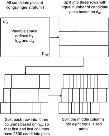
Fig. 1. Visualization of the stratification of candidate plots based on the two ALS variables.
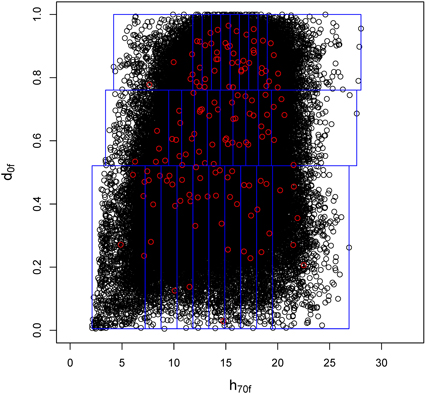
Fig. 2. Example of the use of two laser variables for plot selection in the municipality of Konsvinger in forest stratum IV. The plot shows the five pre-selected candidate plots in each ALS stratum defined by d0f and h70f.
The companies that performed the field inventory were instructed that they were allowed to select only one among the five pre-selected plots for measurement. The reason why they had five plots to choose among was to allow for selecting plots in a cost-effective manner while in field. Thus, approximately 30 plots per forest stratum were measured from both municipalities, and after these data sets were merged, each forest stratum had around 60 plots (Table 1).
GNSS navigator was used to find the pre-defined plot positions. Navigating exactly to the correct position was sometimes challenging due to the changing real-time coordinates given by the GNSS navigator. Arrival alarm was set to trigger at ten meters distance from the destination. Then the person operating the GNSS would record the current position for 30 seconds and then move the remaining distance to the target using a precision compass and a tape measure before recording the final plot coordinates. Despite this precaution, the average distance between predefined and final positions was 5.1 m with a standard deviation of 3.8 m. Thus, the real distribution of measured plots on the pre-defined ALS strata was not identical to the initial design, as the ALS variables used for the stratification change with the distance (Fig. 3). Combined with some practical difficulties experienced in the field, the number of plots in each ALS stratum and municipality could be zero or two instead of one. Fig. 4 depicts the ALS-assisted and ordinary sample plots in a scatter diagram defined by the two stratification variables. The final distribution of plots was relatively similar for forest strata I and IV. For strata II and III the ordinary plot selection actually produced more extreme values, whereas the ALS-assisted plots were more often placed into stands with high canopy density and height.
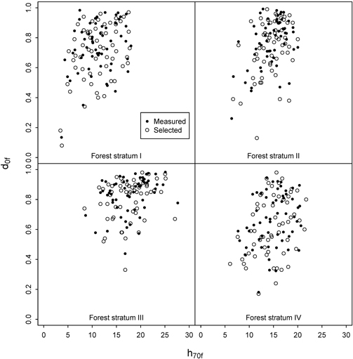
Fig. 3. Distribution of h70f and d0f at the intended sample plots and the plots actually measured in the field for the ALS-assisted data set.
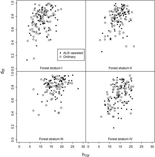
Fig. 4. Distribution of h70f and d0f at the ALS-assisted and ordinary sample plots.
2.3.3 Validation plots
19–20 independent 1000 m2 validation plots (r = 17.84 m) were selected randomly for each of the four forest strata and measured in September 2009. The field measurements and calculations were performed similarly to the other plots, except that 20 sample trees were selected for height measurement. Table 2 displays the stand attributes of the validation plots. When applying the laser-based regression, the size of the application plot should be similar to modeling plot (Magnussen and Boudewyn 1998). Because the validation plots were larger than modeling plots, they were split into four separate 250 m2 sections, for which the regression models were applied. The predictions made for the sub-plots were averaged to obtain a volume estimate for the entire plot.
| Table 2. Summary of the validation data set. hL = Lorey’s mean height, dg = mean diameter by basal area, G = basal area, V = volume. | |||
| Min | Max | Mean | |
| Young forest (forest stratum I) | (n = 19) | ||
| hL (m) | 10.1 | 19.3 | 13.2 |
| dg (cm) | 7.5 | 22.0 | 12.7 |
| G (m2 ha–1) | 6.6 | 35.5 | 20.5 |
| V (m3 ha–1) | 36.1 | 328.1 | 144.6 |
| Spruce (%) | 0 | 99 | 69 |
| Pine (%) | 0 | 100 | 26 |
| Deciduous (%) | 0 | 19 | 5 |
| Mature spruce forest, poor site quality (forest stratum II) | (n = 20) | ||
| hL (m) | 12.0 | 24.8 | 17.9 |
| dg (cm) | 10.2 | 27.1 | 17.5 |
| G (m2 ha–1) | 12.5 | 36.3 | 26.7 |
| V (m3 ha–1) | 82.2 | 389.5 | 236.4 |
| Spruce (%) | 22 | 100 | 76 |
| Pine (%) | 0 | 64 | 15 |
| Deciduous (%) | 0 | 38 | 9 |
| Mature spruce forest, good site quality (forest stratum III) | (n = 20) | ||
| hL (m) | 16.4 | 29.2 | 20.7 |
| dg (cm) | 14.0 | 27.9 | 18.6 |
| G (m2 ha–1) | 18.9 | 49.6 | 34.3 |
| V (m3 ha–1) | 156.2 | 565.0 | 347.1 |
| Spruce (%) | 15 | 100 | 81 |
| Pine (%) | 0 | 82 | 14 |
| Deciduous (%) | 0 | 20 | 6 |
| Mature pine forest (forest stratum IV) | (n = 19) | ||
| hL (m) | 13.8 | 21.6 | 17.0 |
| dg (cm) | 11.6 | 24.3 | 17.4 |
| G (m2 ha–1) | 11.6 | 33.9 | 22.6 |
| V (m3 ha–1) | 80.6 | 323.3 | 188.2 |
| Spruce (%) | 0 | 84 | 25 |
| Pine (%) | 15 | 100 | 74 |
| Deciduous (%) | 0 | 8 | 2 |
2.4 Model construction and accuracy assessment
We used both ordinary (OLS) and partial least squares (PLS) (Wold et al. 1983; Martens 2001) regression to link the laser variables with the reference volumes. The PLS regression is useful when there is a large number of collinear predictor variables, but only a relatively small number of observations. Næsset et al. (2005) compared OLS, PLS, and seemingly unrelated regression models, and found that there were only minor differences between the methods. Normally ordinary least squares are preferred due to simplicity, but in this case we decided to also include PLS, because it enabled fitting the model and application of variable selection algorithm also when the number of plots was reduced down to 15 (see 2.5). The PLS regression is based on singular value decomposition of the original matrix of predictor variables. The orthogonal linear combinations of the original variables pack the essential information of the full the variance-covariance matrix into latent components, which are then used as predictors in the regression. If the original variables are collinear, only a few latent components are needed in the prediction.
We also tested weighted least squares. The weights were derived as the percentage of candidate plots in each of the ALS strata relative to the total number of candidate plots. However, the RMSEs obtained this way were slightly worse than without the weighting and they are not reported.
The statistical software R (R core team 2012) and the external library pls (Mevik and Wehrens 2007) were used to fit the models. The models were fitted separately for each forest stratum, and separately for ordinary and ALS-assisted sample plots. The model shape was based on logarithmic transformations (Eq. 1):
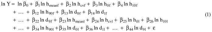
where Y is the reference volume, and the predictor variables are as explained in section 2.2: hmean = mean height of laser echoes from the vegetation (>2 m) (m); hcv = coefficient of variation for the echoes >2 m (%); h0, h10, …,h90 = height percentiles and d0, d1, … , d9 = canopy densities as defined in section 2.3.2, and ε is the random residual term. First and last return variables are indicated by f and l, respectively.
After fitting the initial model, stepwise variable selection was applied to exclude unnecessary predictors from the final OLS model. The rule was that the variables remaining in the model should produce a statistically significant improvement in quality of model fit at p < 0.05. The PLS regression processed the original variables into latent components and returned the root mean square errors (RMSEs) obtained using different numbers of latent components (derived from leave-one-out cross validation). The PLS algorithm is prone to overfitting if too many latent components are selected (Nørgaard et al. 2000), so we restricted the maximum number of latent components to seven. In addition, we did not directly select the same number of latent components that produced the smallest RMSE. Instead, we selected the smallest number of latent components that achieved RMSE smaller than 1.03 × RMSEmin (Næsset et al. 2005).
When applying the fitted models for prediction purposes, the predictions were converted back to arithmetic scale using the exponential transform. The bias induced by this transformation was corrected by adding half of the model residual variance to the prediction before the transformation (Baskerville 1972). The accuracy of the predictions was assessed by means of the relative RMSE and relative mean difference (D) calculated on the original scale (Eq. 2, 3):
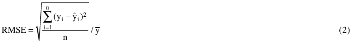
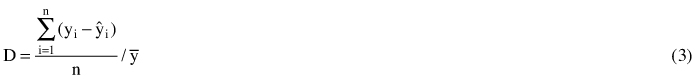
where n is the number of plots, yi is the reference volume at plot i, ŷi is the ALS-based volume prediction, and ![]() is the mean of the reference volumes. The absolute RMSE and D can be calculated by multiplying the relative values by the mean reference volume. In addition, the R2 value was calculated in the original scale as the square of Pearson’s correlation coefficient between the field-estimated and predicted volume. The statistical significance of the D was tested using paired samples t-test between the reference and ALS-estimated volumes.
is the mean of the reference volumes. The absolute RMSE and D can be calculated by multiplying the relative values by the mean reference volume. In addition, the R2 value was calculated in the original scale as the square of Pearson’s correlation coefficient between the field-estimated and predicted volume. The statistical significance of the D was tested using paired samples t-test between the reference and ALS-estimated volumes.
The fitted models were evaluated first based on the RMSE in the modeling data. As we had two separate data sets for modeling, we also made a cross-comparison test where the ordinary model was used to predict volumes in the ALS-assisted data set, and vice versa. However, the final evaluation was based on the model performance in the independent validation data.
2.5 Reducing the number of plots
We also studied how much reducing the number of field plots (sub-sampling) would affect the accuracy using either traditional or ALS-assisted plot selection. It can be assumed that ALS-assisted sub-sampling should have a smaller effect on model precision than random sampling. For the ordinary plots, the sub-sampling was done using simple random sampling into 50, 40, 30, 20 and 15 plots per forest stratum. For the ALS-assisted plots, the reduction was done so that the whole range of ALS strata would be utilized. The data from the two municipalities were pooled into one dataset, and the following sub-sampling rules were applied:
- 50 per forest stratum: Remove a randomly selected plot from each of the ten h70f columns.
- 40 per forest stratum: Remove two randomly selected plots from each of the ten h70f columns. The plots cannot be in the same d0f row.
- 30 per forest stratum: Remove a randomly selected plot from each of the 30 ALS strata defined by the ten h70f columns and the three d0f rows.
- 20 per forest stratum: Merge the ten h70f columns into five new columns. For each of the merged columns, select randomly one of the two original columns, and remove all plots that were in there. In addition, remove two plots from the remaining original column so that at least one plot remains in each d0f row.
- 15 per forest stratum: Same as above, but remove three plots instead of two.
In addition, if the number of plots in some of the ALS strata was smaller than expected due to difficulties in the field work, these ALS strata were not considered in the sub-sampling. The sub-sampling was repeated 300 times, and RMSE and D were calculated at each iteration after refitting the model. Only PLS regression was used in the simulation, because the OLS model variable selection could not be done when the number of plots became smaller than the number of predictors in the initial model (n = 44).
3 Results
3.1 Model performance
The OLS and PLS models fitted for the ordinary and ALS-assisted sample plot data are displayed in Table 3. The R2-values ranged from 0.84 to 0.94, indicating that all models fit reasonably well. In most cases the OLS models had smaller RMSEs than the PLS models. However, the real evaluation between the models must be based on the cross-comparison (Table 4, Fig. 5) and prediction on the separate validation plots (Table 5, Fig. 6).
| Table 3. Predictors selected to each model and their RMSE and R2 in the model data. | |||||||||||
| n | OLS predictors | OLS RMSE (%) | OLS R2 | PLS latent components | PLS RMSE (%) | PLS R2 | |||||
| Young forest (forest stratum I) | |||||||||||
| ALS-assisted plots | 59 | d6f | h90l | d1l | 15.9 | 0.93 | 3 | 18.2 | 0.91 | ||
| Ordinary plots | 72 | hmeanf | d4f | d1l | d9l | 16.0 | 0.92 | 3 | 15.9 | 0.93 | |
| Spruce forest at low fertility sites (forest stratum II) | |||||||||||
| ALS-assisted plots | 59 | h40f | h70f | d4f | h0l | 13.9 | 0.89 | 3 | 14.7 | 0.88 | |
| Ordinary plots | 59 | hcvf | h30f | d3f | d9f | h10l | 14.4 | 0.90 | 3 | 16.0 | 0.87 |
| Spruce forest at high fertility sites (forest stratum III) | |||||||||||
| ALS-assisted plots | 58 | hmeanf | d0f | 14.3 | 0.89 | 3 | 15.6 | 0.87 | |||
| Ordinary plots | 58 | hmeanl | d1l | d5l | 16.7 | 0.88 | 4 | 17.5 | 0.87 | ||
| Pine forest (forest stratum IV) | |||||||||||
| ALS-assisted plots | 59 | d9f | h50l | d2l | d8l | 14.1 | 0.92 | 4 | 13.9 | 0.92 | |
| Ordinary plots | 75 | hmeanf | d0f | d7l | 21.4 | 0.84 | 4 | 19.9 | 0.86 | ||
| Table 4. Relative RMSE and D between the reference and predicted volume in a cross-comparison test. | |||||||||
| Method | Stratum | Laser-assisted model, ordinary plots | Ordinary model, laser-assisted plots | ||||||
| n | Mean volume | RMSE% | D% | n | Mean volume | RMSE% | D% | ||
| OLS | I | 72 | 140.2 | 17.9 | 3.5 | 59 | 155.0 | 16.7 | 2.5 |
| II | 59 | 211.2 | 21.5 | 3.1 | 59 | 230.3 | 22.5 | 1.7 | |
| III | 58 | 262.5 | 18.5 | 0.6 | 58 | 332.8 | 17.1 | 2.9 | |
| IV | 75 | 196.3 | 27.3 | 2.0 | 59 | 186.0 | 20.9 | 5.8* | |
| PLS | I | 72 | 140.2 | 18.8 | –4.4* | 59 | 155.0 | 18.7 | 4.9* |
| II | 59 | 211.2 | 20.6 | 1.2 | 59 | 230.3 | 18.9 | –2.0 | |
| III | 58 | 262.5 | 18.4 | –0.1 | 58 | 332.8 | 16.7 | 3.5 | |
| IV | 75 | 196.3 | 25.0 | 3.7 | 59 | 186.0 | 23.7 | –4.0 | |
| *Mean difference statistically significant at p = 0.05 | |||||||||
| Table 5. Relative RMSE and D between the reference and predicted volume in the validation plots. | |||||||
| Method | Stratum | n | Mean volume | Laser-assisted model | Ordinary model | ||
| RMSE% | D% | RMSE% | D% | ||||
| OLS | I | 19 | 144.6 | 15.3 | 2.7 | 15.1 | 4.9 |
| II | 20 | 236.4 | 14.0 | 1.6 | 15.6 | 4.3 | |
| III | 20 | 347.1 | 15.7 | 8.4* | 16.9 | 10.4* | |
| IV | 19 | 188.2 | 17.3 | 1.7 | 17.0 | 2.9 | |
| PLS | I | 19 | 144.6 | 15.3 | 1.7 | 16.3 | 5.6 |
| II | 20 | 236.4 | 14.3 | 2.6 | 13.8 | 0.4 | |
| III | 20 | 347.1 | 15.8 | 6.8 | 17.2 | 9.9* | |
| IV | 19 | 188.2 | 18.2 | 3.1 | 16.8 | 2.1 | |
| *Mean difference statistically significant at p = 0.05 | |||||||
First, there were no clear differences between OLS and PLS regressions. For the validation plots (Table 5), OLS performed better, as the PLS models had clearly smaller RMSE than OLS only for the ordinary plots in forest stratum II. In the cross-comparison however, the PLS had smaller RMSE in five out of eight cases (Table 4). For the validation plots the maximum difference in RMSE between the two methods was 1.8 percent points, but in other cases much smaller (0.0–1.2 percent points). Based on these results, there was no reason to use PLS instead of the simpler OLS. Thus, in the following we focus on the OLS results, but PLS was still needed in the sub-sampling experiment (section 3.2).
For forest stratum I (young forest), the ordinary OLS model achieved slightly smaller RMSE than the ALS-assisted model both in cross-comparison (16.7% vs. 17.9%) and at the independent validation plots (15.1% vs. 15.3%). However, the differences were relatively small, and in the validation plots the ordinary model had slightly larger mean difference. It is notable that the ordinary model was based on 72 plots and four predictors, whereas the ALS-assisted model was fitted using 59 plots and had three predictors, and both had equal accuracy in the modeling data (Table 3). Both data sets had a similar range in reference volume and other stand attributes (Table 1). Thus, the ALS-assisted model obtained similar accuracy as the ordinary model with fewer field plots.
For forest stratum II (spruce forest on poor sites), both data sets had 59 plots, and the OLS models had four or five predictors. This time the model fitted using the ALS-assisted data had slightly smaller RMSE than the ordinary model both in the cross-comparison (RMSE = 21.5% vs. 22.5%) and the validation data (RMSE = 14.0% vs. 15.6%). The ALS-assisted data set had more plots with higher reference volumes (Fig. 5), which decreased the number of outliers. Interestingly, the PLS model for ordinary plots was somewhat better than the OLS model both in the cross-comparison and at the validation plots.
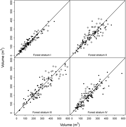
Fig. 5. Cross-comparison of the OLS models. Black = predictions for ordinary plots using the ALS-assisted model, white = prediction for ALS-assisted plots using ordinary model.
The ordinary OLS model fitted for forest stratum III (spruce forest on fertile sites) had three predictors, while the ALS-assisted model used only two. Both data sets had 58 plots evenly distributed across the volume range occurring in the region, but the ALS-assisted data set had again slightly more plots from the high end of the volume range (Fig. 4). Visual inspection of the residual diagrams showed that the models fitted into ordinary data (RMSE = 16.7%) had somewhat more outliers than the models fitted into ALS-assisted data (RMSE = 14.3%). In the cross-comparison test, the ALS-assisted model produced higher RMSEs in the ordinary data (RMSE = 18.5%) than the ordinary model in the ALS-assisted data (RMSE = 17.1%). Because of the outliers, the ordinary data set had higher RMSEs in both model fitting and application. However, in the independent validation data the ALS-assisted model had smaller RMSE (15.7% vs. 16.9%). This stratum was the only case where the mean differences were statistically significant in the validation plots. Volume was overestimated by both models, but slightly more by the ordinary model (10.4% vs. 8.4%) (Fig. 6).
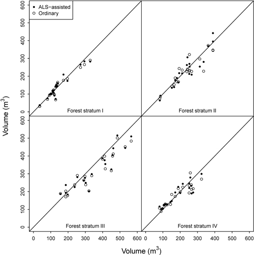
Fig. 6. OLS model predictions for the validation plots.
In the case of forest stratum IV (pine forest), the initial OLS model with ALS-assisted plots (four predictors, RMSE = 14.1%) had again considerably smaller RMSE than the ordinary OLS model (three predictors, RMSE = 21.4%) (Table 3). The residual diagram again indicated more scatter in the ordinary data set, and thus in the cross-comparison the results reversed (ALS-assisted model RMSE in the ordinary data 27.3% vs. ordinary model RMSE in the ALS-assisted data 20.9%). However, in the independent validation plots the differences between the two models were marginal (Table 5). In the cross-comparison, the t-test indicated a statistically significant difference between the estimates obtained from the ordinary model and the field-measured values (5.8%), and also in the validation plots the mean difference was slightly larger for the ordinary model. Thus, the ALS-assisted model fitted with 59 plots should be a more viable choice than the ordinary model that used 75 plots.
3.2 Reducing the number of plots
The reduction of the number of plots was simulated with both data sets using PLS to evaluate (using the validation plots) if the ALS-assisted plot selection would be less sensitive to the size of the modeling data (Table 6). The results showed that the laser-assisted plot selection became more competitive when the number of plots decreased. When the number of plots decreased to 30, the RMSE was better for laser-assisted plots in forest strata I, III, and IV. When only 15 plots were used, the laser-assisted model was better in all cases. Also the mean difference was considerably lower for ALS-assisted models in forest strata I and III. Using the ALS-assisted sub-sampling, the number of plots could be reduced from 60 to 40 without increasing the RMSE by more than one percent point.
| Table 6. Results of reducing the number of plots by sub-sampling. The RMSE and D are PLS averages after 300 iterations. | |||||||||
| n | Forest stratum I | Forest stratum II | Forest stratum III | Forest stratum IV | |||||
| RMSE (%) | D (%) | RMSE (%) | D (%) | RMSE (%) | D (%) | RMSE (%) | D (%) | ||
| ALS-assisted | All | 15.3 | 1.7 | 14.3 | 2.6 | 15.8 | 6.8 | 18.2 | 3.1 |
| 50 | 15.3 | 1.6 | 14.9 | 2.3 | 16.0 | 6.4 | 18.1 | 2.6 | |
| 40 | 16.0 | 2.2 | 15.0 | 1.7 | 16.7 | 5.8 | 18.1 | 2.0 | |
| 30 | 15.9 | 2.1 | 16.2 | 1.3 | 17.0 | 6.2 | 18.7 | 2.4 | |
| 20 | 16.6 | 3.4 | 17.2 | 1.3 | 18.6 | 5.8 | 19.7 | 1.5 | |
| 15 | 17.1 | 2.9 | 17.5 | 1.2 | 19.2 | 6.0 | 20.0 | 1.6 | |
| Ordinary | All | 16.3 | 5.6 | 13.8 | 0.4 | 17.2 | 9.9 | 16.8 | 2.1 |
| 50 | 16.6 | 5.0 | 14.0 | 0.1 | 17.0 | 9.3 | 17.7 | 2.0 | |
| 40 | 17.2 | 5.4 | 14.8 | –0.5 | 17.1 | 8.9 | 18.4 | 1.4 | |
| 30 | 17.5 | 5.1 | 15.5 | –0.2 | 18.4 | 9.3 | 19.1 | 0.8 | |
| 20 | 18.3 | 6.0 | 16.6 | 0.3 | 19.5 | 9.0 | 21.0 | –0.4 | |
| 15 | 20.7 | 5.9 | 18.4 | 0.3 | 21.1 | 9.1 | 22.6 | –0.4 | |
4 Discussion
Both the ALS-assisted and the ordinary sample plot selection produced reasonably good coverage of the range of values of the ALS metrics used for stratification and thus the differences between the models were relatively small. Considering only OLS results, the ALS-assisted models were clearly better for forest stratums II and III. For stratums I and IV the precision was practically equal, but the ordinary data sets were 13 and 15 plots larger, respectively. Also the validation plot mean differences between reference and ALS-estimated volumes were constantly higher for the ordinary models. The sub-sampling test indicated better performance with the ALS-assisted data set. Thus ALS-assisted selection of sample plots should help to reduce the inventory costs, if the practical constraints can be overcome.
However, the differences between the two data sets were small. In some cases the results changed when PLS was used instead of OLS. The reason for the changes might be the varying success in variable selection (or selecting the number of latent components), i.e. that the change of method with best performance was caused by a somewhat different variable selection rather than by method as such. For example for forest stratum IV, the ALS-assisted model had higher RMSE for the validation plots using PLS with four latent components than OLS with four predictors. However, if three latent components were used with the PLS (against the algorithm), the RMSEs would have been equal. In a practical application this would have remained unknown. The variable selection with OLS seemed to function reliably, as the PLS method provided better RMSE for the validation plots only in one out of eight cases. Thus, there should usually be no need to use PLS instead of OLS.
Earlier studies have also confirmed the utility of the ALS-assisted plot selection. Hawbaker et al. (2009) modeled the biomass of coniferous and deciduous forests and found that random plot selection produced 41–47% larger RMSE than the ALS-assisted plot selection in the independent validation plots. Hence, in other circumstances the gain of ALS-assisted model selection can be considerably larger than in our case. Maltamo et al. (2011) tested a reduction in sample size based on two ALS variables for stratification in a manner similar to ours, and found that the decrease from 181 to 61 plots did not significantly change the volume estimated using k-MSN imputation. However, their results are not directly comparable to ours as they used non-parametric imputation, which is more sensitive to the size of the training data set than regression analysis. Other results (Dalponte et al. 2011; Junttila et al. 2013) also indicate that 40–50 carefully placed plots should be enough for regression-based estimation. Our results are similar, as the number of plots could be reduced down to 40 with only a minor increase in RMSE (0.1–0.9 percentage points) using the ALS-assisted sub-sampling.
Our ALS-assisted plot selection approach was based on two ALS variables and the division of study area into 30 ALS strata (three density classes, ten height classes within each density class). This is a simple method for confirming that the variable space is covered evenly. The number and width of rows and columns can be adjusted according to the number of plots that are measured in the field, as long as the even coverage is retained. Our method was relatively conservative in that the extreme values occurring in the data had a relatively small probability of being selected (Fig. 2). Defining the extreme classes differently would have enabled higher inclusion probabilities for the extreme values. This could be useful if nearest neighbor methods are used, as the neighbor database should also enable estimation of high ends of the scale, but in case of linear regression such observations may have a considerable influence on the model parameters (Cook 1977). Junttila et al. (2013) and Grafström and Ringvall (2013) describe more advanced methods for plot selection, but our results indicate that even a simple method should improve the results compared with simple random sampling.
We propose that the stratification should be based on one ALS-based canopy height and one canopy density variable. Different height and density variables are highly correlated, so the end result should not be sensitive to which two of the alternative variables are chosen. A common practice is however to use the variables that approximate mean height and canopy cover at the plot; in our case these were h70f and d0f, respectively.
All in all, the method has plenty of room for customization, as different column and row numbers, as well as different stratification variables could be tested. However, testing the multiple alternatives should be done using simulation, because measuring even two independent data sets in the field is very expensive. We only considered the volume here, but it should be noted that similar stratification should function also in the estimation of other forest attributes, such as mean height, mean diameter, and basal area.
Despite the good results, the application of this method has some practical challenges. The cost savings depend on how smoothly the ALS-assisted plot selection can be implemented by the forest inventory companies. First, the ALS data set must be processed and analyzed for plot positioning before the field work can start. This is primarily computational work and should be easily automatized. Sometimes bad weather can delay the ALS data acquisition, while the field measurements cannot usually be delayed as they are laborious and should ideally be finished within the same year as the scanning. Also the ALS data processing must be very quick and without any problems to stay in the schedule. Furthermore, the GNSS inaccuracies mean that the distribution of measured plots on the ALS strata is not exactly such as planned in the design phase. We also allowed the inventory companies to select the measured plot out of five alternatives and thus our ALS-assisted data set may not fulfill all criteria of a pure probability sample. Third, it takes some time until the practical organizations and companies will accept and adapt to the new methodology, and errors are likely to occur during the transition period. This problem is to be expected at least in Norway, where the practical work is carried out by several inventory companies, whose working procedures have remained largely unchanged since the introduction of the area-based method in 2002. For the current study however, the feedback from the inventory companies was that field work required by the ALS-assisted plot selection was no more laborious than the standard cluster sampling.
In the near future, it will also be possible to use existing ALS data from previous acquisitions as a basis for plot selection in new inventories. This approach may not be as accurate as using up-to-date data but should be much more easily arranged in practice, and should be investigated in the future studies.
Acknowledgements
This study was supported by the Skogtiltaksfondet, Innovation Norway, Mjøsen Skog SA, Foran Norge AS, Norwegian University of Life Sciences, and the strategic funds of the University of Eastern Finland.
References
Baskerville G.L. (1972). Use of logarithmic regression in the estimation of plant biomass. Canadian Journal of Forest Research 2: 49–53. http://dx.doi.org/10.1139/x72-009.
Braastad H. (1966). Volume tables for birch. Meddelelser fra Det Norske Skogforsøksvesen 21: 23–78. [In Norwegian with English summary].
Brantseg A. (1967). Volume functions and tables for Scots pine. South Norway. Meddelelser fra Det Norske Skogforsøksvesen 22: 689–739. [In Norwegian with English summary].
Cook R.D. (1977). Detection of influential observations in linear regression. Technometrics 19(1): 15–18. http://dx.doi.org/10.2307/1268249.
Dalponte M., Martinez C., Rodeghiero M., Gianelle D. (2011). The role of ground reference data collection in the prediction of stem volume with LiDAR data in mountainous areas. ISPRS Journal of Photogrammetry and Remote Sensing 66: 787–797. http://dx.doi.org/10.1016/j.isprsjprs.2011.09.003.
Esseen P.-A., Ehnström B., Ericson L., Sjöberg K. (1997). Boreal forests. Ecological Bulletins 46: 16–47. http://www.jstor.org/stable/20113207.
Fitje A., Vestjordet E. (1977). Stand height curves and new tariff tables for Norway spruce. Reports of the Norwegian Forest Research Institute 34: 23–62. [In Norwegian with English summary]
Gobakken T., Næsset E. (2008). Assessing effects of laser point density, ground sampling intensity, and field sample plot size on biophysical stand properties derived from airborne laser scanner data. Canadian Journal of Forest Research 38(5): 1095–1109. http://dx.doi.org/10.1139/X07-219.
Grafström A., Ringvall A.H. (2013) Improving forest field inventories by using remote sensing data in novel sampling designs. Canadian Journal of Forest Research 43(11): 1015–1022. http://dx.doi.org/10.1139/cjfr-2013-0123.
Hawbaker T.J., Keuler N.S., Lesak A.A., Gobakken T., Contrucci K., Radeloff V.C. (2009). Improved estimates of forest vegetation structure and biomass with a LiDAR-optimized sampling design. Journal of Geophysical Research 114, G00E04. http://dx.doi.org/10.1029/2008JG000870.
Holmgren J. (2004). Prediction of tree height, basal area and stem volume in forest stands using airborne laser scanning. Scandinavian Journal of Forest Research 19: 543–553. http://dx.doi.org/10.1080/02827580410019472.
Jensen J.L.R., Humes K.S., Conner T., Williams C.J., DeGroot J. (2006). Estimation of biophysical characteristics for highly variable mixed-conifer stands using small-footprint lidar. Canadian Journal of Forest Research 36: 1129–1138. http://dx.doi.org/10.1139/x06-007.
Junttila V., Finley A.O., Bradford J.B., Kauranne T. (2013). Strategies for minimizing sample size for use in airborne LiDAR-based forest inventory. Forest Ecology and Management 292: 75–85. http://dx.doi.org/10.1016/j.foreco.2012.12.019.
Magnussen S., Boudewyn P. (1998). Derivations of stand heights from airborne laser scanner data with canopy-based quantile estimators. Canadian Journal of Forest Research 28: 1016–1031. http://dx.doi.org/10.1139/x98-078.
Magnussen S., Næsset E., Gobakken T. (2010). Reliability of LiDAR derived predictors of forest inventory attributes: a case study with Norway spruce. Remote Sensing of Environment 114: 700–712. http://dx.doi.org/10.1016/j.rse.2009.11.007.
Maltamo M., Bollandsås O.M., Vauhkonen J., Breidenbach J., Gobakken T., Næsset E. (2011). Different plot selection strategies for field training data in ALS-assisted forest inventory. Forestry 84: 23–31. http://dx.doi.org/10.1093/forestry/cpq039.
Martens H. (2001). Reliable and relevant modelling of real world data: a personal account of the development of the development of PLS regression. Chemometrics and Intelligent Laboratory Systems 58: 85–95.
Mevik B.-H., Wehrens R. (2007). The pls package: principal component and partial least squares regression in R. Journal of Statistical Software 18(2): 1–24.
Næsset E. (2002). Predicting forest stand characteristics with airborne scanning laser using a practical two-stage procedure and field data. Remote Sensing of Environment 80: 88–99. http://dx.doi.org/10.1016/S0034-4257(01)00290-5.
Næsset E. (2004). Practical large-scale forest stand inventory using a small-footprint airborne scanning laser. Scandinavian Journal of Forest Research 19: 164–179. http://dx.doi.org/10.1080/02827580310019257.
Næsset E., Gobakken T. (2008). Estimation of above- and below-ground biomass across regions of the boreal forest zone using airborne laser. Remote Sensing of Environment 112: 3079–3090. http://dx.doi.org/10.1016/j.rse.2008.03.004.
Næsset E., Gobakken T., Holmgren J., Hyyppä H., Hyyppä J., Maltamo M., Nilsson M., Olsson H., Persson Å., Söderman U. (2004). Laser scanning of forest resources: the Nordic experience. Scandinavian Journal of Forest Research 19: 482–499. http://dx.doi.org/10.1080/02827580410019553.
Næsset E., Bollandsås O.M., Gobakken T. (2005). Comparing regression methods in estimation of biophysical properties of forest stands from two different inventories using laser scanner data. Remote Sensing of Environment 94: 541–553. http://dx.doi.org/10.1016/j.rse.2004.11.010.
Nørgaard L., Saudland A., Wagner J., Pram Nielsen J., Munck L., Engelsen S.B. (2000). Interval partial least-squares regression (iPLS): a comparative chemometric study with an example from near-infrared spectroscopy. Applied Spectroscopy 54: 413–419.
Packalén P., Maltamo M. (2007). The k-MSN method for the prediction of species-specific stand attributes using airborne laser scanning and aerial photographs. Remote Sensing of Environment 109: 328–341. http://dx.doi.org/10.1016/j.rse.2007.01.005.
R Core Team (2012). R: A language and environment for statistical computing. R Foundation for Statistical Computing, Vienna, Austria. ISBN 3-900051-07-0. http://www.R-project.org/.
Reutebuch S.E., McGaughey R.J., Andersen H.-E., Carson W.W. (2003). Accuracy of a high-resolution lidar terrain model under a conifer forest canopy. Canadian Journal of Remote Sensing 29: 527–535. http://dx.doi.org/10.5589/m03-022.
Särndal C.-E., Swensson B., Wretman J. (1992). Model assisted survey sampling. Springer-Verlag, New York. 694 p.
Vestjordet E. (1967). Functions and tables for volume of standing trees. Norway spruce. Meddelelser fra Det Norske Skogforsøksvesen 22: 539–574. [In Norwegian with English summary].
Vestjordet E. (1968). Merchantable volume of Norway spruce and Scots pine based on relative height and diameter at breast height or 2.5 m above stump level. Meddelelser fra Det Norske Skogforsøksvesen 25: 411–459. [In Norwegian with English summary].
Wehr A., Lohr U. (1999). Airborne laser scanning – an introduction and overview. ISPRS Journal of Photogrammetry & Remote Sensing 54: 68–82. http://dx.doi.org/10.1016/S0924-2716(99)00011-8.
Wold S., Martens H., Wold H. (1983). The multivariate calibration problem in chemistry solved by the PLS method. In: Ruhe A., Kågström B. (eds.). Matrix pencils. Springer Verlag, Heidelberg. p. 286–293.
Total of 32 references
