Mika Aalto  ,
Olli-Jussi Korpinen,
Tapio Ranta
,
Olli-Jussi Korpinen,
Tapio Ranta
Feedstock availability and moisture content data processing for multi-year simulation of forest biomass supply in energy production
Aalto M., Korpinen O.-J., Ranta T. (2019). Feedstock availability and moisture content data processing for multi-year simulation of forest biomass supply in energy production. Silva Fennica vol. 53 no. 4 article id 10147. https://doi.org/10.14214/sf.10147
Highlights
- A method for allocating forest biomass availability for a multi-year simulation model was developed
- The possibility to take the quality change of feedstock into account by moisture estimations was studied
- A method to estimate weather data for moisture estimation equations with fewer parameters was presented.
Abstract
Simulation and modeling have become more common in forest biomass studies. Dynamic simulation has been used to study the supply chain of forest biomass with numerous different models. A robust predictive multi-year model requires biomass availability data, where annual variation is included spatially and temporally. This can be done by using data from enterprises, but in some cases relevant data is not accessible. Another option is to use forest inventory data to estimate biomass availability, but this data must be processed in the correct form to be utilized in the model. This study developed a method for preparing forest inventory data for a multi-year simulation supply model using the theoretical availability of feedstock. Methods for estimating quality changes during roadside storage are also presented, including a possible parameter estimation to decrease the amount of data needed. The methods were tested case by case using the inventory database “Biomass Atlas” and weather data from a weather station in Mikkeli, Finland. The data processing method for biomass allocation produced a reasonable quantity of stands and feedstock, having a realistic annual supply with variation for the demand point. The results of the study indicate that it is possible to estimate moisture content changes using weather data. The estimations decreased the accuracy of the model and, therefore, estimations should be kept minimal. The presented data preparation method can generate a supply of forest biomass for the simulation model, but the validity of the data must be ensured for correct model behavior.
Keywords
bioenergy;
simulation;
forest resources;
data analysis;
geographic information system
-
Aalto,
Lappeenranta-Lahti University of Technology LUT, School of Energy Systems, Laboratory of Bioenergy, Lönnrotinkatu 7, FI-50100 Mikkeli, Finland
 https://orcid.org/0000-0002-7768-1145
E-mail
mika.aalto@lut.fi
https://orcid.org/0000-0002-7768-1145
E-mail
mika.aalto@lut.fi
- Korpinen, Lappeenranta-Lahti University of Technology LUT, School of Energy Systems, Laboratory of Bioenergy, Lönnrotinkatu 7, FI-50100 Mikkeli, Finland E-mail olli-jussi.korpinen@lut.fi
-
Ranta,
Lappeenranta-Lahti University of Technology LUT, School of Energy Systems, Laboratory of Bioenergy, Lönnrotinkatu 7, FI-50100 Mikkeli, Finland
https://orcid.org/0000-0001-5464-5136
E-mail
tapio.ranta@lut.fi
Received 29 January 2019 Accepted 17 October 2019 Published 22 October 2019
Views 78696
Available at https://doi.org/10.14214/sf.10147 | Download PDF

1 Introduction
Forest biomass use has great potential to decrease the use of fossil fuel, as it can be delivered in all forms needed and it is considered carbon dioxide neutral (Demirbas et al. 2009). In addition, it can be utilised in rural areas (Wasajja and Chowdhury 2017) and contribute significantly to the national energy supply. The long-term availability of forest biomass is a concern, but proper management may ensure it in cases of higher demand (Nabuurs et al. 2007). To make full use of the long lifespan of the power plants, the forest biomass supply must be secured for years to come.
The forest biomass supply chain is a complex system (Rentizelas et al. 2009). Its main activities include harvesting, extraction, roadside storage, processing, transportation and conversion operations. Processing may be done at an early stage, such as roadside chipping, or after transportation as chipping at the end user site, or between transport operations, such as chipping at the terminal. The interactions of machines and random events in the supply chain may cause delays (Asikainen 1995), leading to activities affecting subsequent one in the chain. For these reasons, simulation studies are widely employed (Eriksson et al. 2014b; Väätäinen et al. 2005; Mobini et al. 2011; Aalto et al. 2018; Windisch et al. 2015; Ziesak et al. 2004).
To model a realistic forest biomass supply dynamically, feedstock must be scattered temporally and spatially. The values for each simulated year must vary. The forest biomass supply chain may be studied with dynamic simulation if the available supply of the forest biomass is known.
Previous studies have applied different stochastic methods to simulate available feedstock in different ways. Mobini et al. (2011) have used the shelf-life model that was developed by MacDonald et al. (2007) and estimated the volumes, areas and yield of the stands at the start of the simulation year. Mobini et al. (2011) have also used weather conditions, but only for the delays of operations. This method allows for variation in supply volumes, but the locations of the stands do not change. Eriksson et al. (2014b) have generated random supply locations with random parameters. This generates spatial variation but does not include real-life limitations. A model presented by Ziesak et al. (2004) simulated all trees in a stand with their own parameters. The model needs data on the stand and each individual tree. This method can be utilized for small numbers of stands, as it requires a higher amount of computational power, but for hundreds of stands annually, this method would be impractical. Aalto et al. (2018) and Väätäinen et al. (2005) excluded most of the supply chain and included only feedstock arriving at the plant in trucks at different arrival intervals. This is possible, as the studies focused only on the power plant yard operations.
One way to acquire supply information is to use enterprise data, as was done by Windisch et al. (2015). This allows the use of empirical data for different scenarios. However, as enterprise data is not always available, the supply may also be estimated by using databases (e.g. LUKE 2018a; Datta et al. 2017). Nevertheless, this data must be processed for the simulation in order for it to represent values that are as close to real life as possible. It is also noteworthy that spatial analysis of the forest inventory may include errors (Islam et al. 2012; Holopainen et al. 2010), and therefore, the data requires validation.
There is a lack of dynamic methods for forest biomass supply generation including temporal and spatial features for multi-year simulation models. In addition, possible methods to take into account feedstock quality changes during storage are investigated, as the quality of the feedstock has a considerable impact on energy production.
In Finland, the forest biomass for energy use is normally left in the stand to dry after harvesting. After that, the biomass is forwarded to the roadside for further transportation to the demand site. Dry biomass is preferred in energy usage, as the moisture content affects the energy density of the biomass (Alakangas et al. 2016).
Modeling the drying process at the roadside storage is an easier option compared to the frequent measuring of the storage. Fixed drying functions have been developed (Sikanen et al. 2013), but they do not take local weather conditions or annual changes into consideration. Measuring would produce more accurate results, but supply forecast simulations cannot use measurements, making the estimation of drying a better option. The effect of the moisture content may be studied by examining different moisture levels of biomass (Kanzian et al. 2016; Eriksson et al. 2014a). However, this results in more simulation runs, which increases the computational load of the model significantly. This may be impractical, as dynamic simulations already call for increased computing power.
Employing statistics to distribute forest inventory data stochastically in terms of space and time allows the more realistic distribution of stands. The spatial allocation of the supply affects the transportation costs, which have an important effect on the total costs of biomass (Allen et al. 1998a). Although estimations increase assumptions that may decrease the validity of the model, they also enable developing the model without numerous or impossible measurements.
As the biomass quality changes during storage and the moisture content is the most significant quality parameter in the energy use of biomass (Alakangas et al. 2016), the option to use moisture estimation equations in the simulation model was studied. Drying speed is highly affected by weather – evaporation, precipitation, humidity, temperature, solar radiation and wind conditions being important parameters. (Routa et al. 2015a). Since simulation models generally study the future impact, the weather is unknown. One option is to use long-term weather forecasting and another is to use historical weather data to create an annual cycle. Annual changes can be considered by stochastically selecting different years to simulate the weather.
This study aims to develop a new data processing method for allocating biomass availability annually with spatial and temporal variation by using a forest inventory database for a multi-year simulation model including biomass moisture content estimation based on local meteorological data. Data allocation with GIS allows the use of real locations if this data is available, or the distribution of availability to the grid points. This enables road and local restrictions (water bodies, extraction distance, etc.) for supply points. Moisture estimation equations need a great number of initial values, some of which are difficult to find. Therefore, this study investigated different possibilities to use moisture estimations: two moisture estimation equations and a simplified equation to acquire evaporation, which is one of the main values of the estimation equation. Moisture estimation equations and a simplified equation for evaporation allow the simulation model to estimate the moisture for the stands, taking both weather and location into account.
2 Material and methods
The Geographical Information System (GIS) was used to create a supply point grid covering a predetermined supply region for a forest biomass supply network that takes into consideration temporal and spatial variety in the supply area and in feedstock drying. The required parameters for drying models were estimated based on local weather data.
2.1 Feedstock availability data
The data for this study was acquired from the biomass inventory database “Biomass Atlas” (LUKE 2018a), but any forest inventory based estimates about theoretical availability may be employed. The data was processed by allocating the availability in the centroids of the supply point grid of a given supply area. The grid dimensions depend on the availability of data, the size of the supply area, and the purpose of the simulation model. This study utilized a 2 km × 2 km grid, and the maximum supply distance was set to 120 km. A total of 3883 stand locations were generated with an annual supply of 78 500 m3 of small diameter trees as whole trees and delimbed trees.
The number of stands in the model should be selected so that they result in a realistic number of points, meaning that the annual number of stands in the supply area should be reasonable. In this case, the stands are in the hundreds rather than thousands, as was the number of centroids in the supply grid. Too large a number of points would lead to the amount of biomass being too low at one point, and too small a number generates amounts of biomass that are too high per point. A reasonable number of annually generated stands is affected by the density of the grid and the extent of the supply area. If all potential availability of the database is utilized, the number of annual stands can be determined by dividing the total availability volume with the estimated average amount of feedstock in one stand. If availability is modified, the number of stands may be determined by Eq. 1.
The sum of the feedstock volume (the unit depends on the units used in the database; the case study uses m3) at one stand (Vsp) for the overall total number of stands (Nsp) is divided by the region’s statistical average (or estimated) volume of the feedstock (unit same as Vsp) at one stand (Vsp,avg). This gives the number of stands that should be used in the model (nsp), but nsp must be less than Nsp.
Because only nsp stands are created annually, the total amount of supply is reduced. This should be taken into account by increasing the available supply of one point. The increase is a ratio of all stands and selected stands (Eq. 2).

Vmsp,i is the feedstock amount at a stand in the model, while Vsp,i is the feedstock amount from the database. With this increase, the annual supply should remain close to the statistical value acquired from the database. As stands are stochastically selected, and some variation will occur in the total amount of the supply, and as the location of the supply changes, in the total transportation distances.
Feedstock information is static data that gives annual amounts, and the harvesting times of stands must be integrated into the data to obtain the annual variations. To this end, statistical data may be used to stochastically schedule harvesting. This study case examines statistics from Finland (LUKE 2018b). A monthly proportion of harvesting is used as the probability of harvesting in a particular month (Eq. 3).
![]()
P(Mi) is the probability of harvesting in month i and Hi is a statistical proportion of harvesting in month i. This allocates the month of the harvest to a regional statistic value, but the harvesting may involve stand-specific limitations. Certain stands can be harvested only during the winter when the ground is frozen. Other stands, usually situated on harder ground, can be harvested in the summer, but not during the thawing period. If stands are located on hard ground and they are near the road, they can be harvested at any time. Harvesting limitations can be taken into account by allocating the probability of harvesting months of the stands with weather conditions to other months by location-specific factors. The day of the harvesting can be reasonably assumed to be uniformly distributed. However, this assumption excludes the reduced amount of work on weekends and public holidays.
To test the method, an estimation of 200 harvested stands were allocated in the supply area. As one set of 200 points represents one year of supply, 30 repetitions were constructed to see the variation between years. The transportation distance was estimated based on the road network generated with GIS. The OpenStreetMap road database (OpenStreetMap contributors 2018) yielded the road network, and driving distances were estimated based on the shortest paths. The average distance was determined according to routes from selected stands to the demand point, located in the middle of the supply area, and compared to the average distance from all the stands to the demand point.
2.2 Drying models
Different drying estimates have been created for forest biomass (Routa et al. 2015b; Liang et al. 1996; Gigler et al. 2000; Erber et al. 2012; Murphy et al. 2012; Kim and Murphy 2013; Heiskanen et al. 2014). Routa et al. (2015b) have validated a model for stem wood at a roadside storage. The model uses a coefficient for evaporation (in mm) and precipitation (in mm) difference and adds a constant to obtain the daily moisture change (Eq. 4). The coefficient and constant are based on storage and wood type. These need to be estimated case specifically.
![]()
Heiskanen et al. (2014) have developed a model that estimates the moisture content with coefficients for both evaporation and precipitation. The moisture content at time i is calculated with Eq. 5.
![]()
The moisture content at time i+1 (wi+1) is estimated by adding the affected drying to moisture content at time i (wi). Drying is estimated with the effect of precipitation and evaporation. Affecting precipitation (P, in mm) is estimated by the difference between the moisture content and equilibrium moisture content (weq), as this difference is scaled by how much the wood can take in moisture. Constant b is added to the divisor. The result of the division is scaled with coefficient a. The evaporation (E, in mm) estimation is also scaled with the difference of moisture and the equilibrium moisture content. Evaporation is multiplied by this difference and the coefficient c. The coefficients a, b, and c are storage and wood type specific and need to be estimated for each case.
Evidently, there are common variables in the moisture prediction models, as all forecast the same phenomenon (Awadalla et al. 2004; Liang et al. 1996; Plumb et al. 1985). Drying estimation equations use precipitation values that are often measured as meteorological data, but evaporation measurements are rarer. Evaporation may be estimated with the Penman-Monteith equation (Eq. 6) (Monteith 1981; Allen et al. 1998b) if no measured data is available.
Eq. 6 uses net irradiance (Rn, in W m–2), ground heat flux (G, in W m–2), dry air density (ρa , in kg m–3), the specific heat capacity of air (cp, in J kg–1 K–1), the vapor pressure deficit of air (es-ea, in Pa), the rate of change of saturation specific humidity with air temperature (Δ, in Pa K–1), the psychrometric constant (γ, in Pa K–1), and surface and aerodynamic resistances (rs and ra, in s m–1) to calculate the energy rate of water evaporation (E, in g s–1m–2) multiplied with the latent heat of vaporization (λ, in J g–1). Due to complications and the need for several parameters, this equation has been simplified in many different ways (Linacre 1977; Salama et al. 2015; Gallego-Elvira et al. 2012). Linacre (1977) simplified Eq. 6 to the form of Eq. 7:
![]()
Eq. 7 uses elevation (Tm = T + 0.006h, h is the elevation (m) (Linacre 1977)), mean temperature (T, in °C), latitude (A, in degrees), and the mean dew-point (Td, in °C) to obtain the evaporation rate (E0, in mm day–1). Most of these parameters are easily acquired from local weather station data. If the mean dew-point cannot be acquired, it may be estimated with Eq. 8 (Linacre 1977):
![]()
This includes R as a daily range of temperature and Rann as the difference between the mean temperatures of the coldest and hottest months (values in °C). These values are easy to acquire from weather data.
Eq. 7 gives net evaporation at the lake that must be scaled to represent the evaporation from on-ground biomass. To do this, a factor can be assigned to scale the evaporation to the correct situation. This factor is an equivalent of the pan coefficient (Ep), which is used to convert the measured evaporation from the pan to the evaporation from crops (Allen et al. 1998b). As roadside storages are situated near the forest and evaporation is from a wood surface, an estimation of 0.5 for Ep is reasonable.
To test the validity of evaporation estimations, Eq. 7 with the pan coefficient 0.5 and polynomial fit for cumulative evaporation developed by Heiskanen et al. (2014) (Eq. 9, later called the VTT equation) were compared with data measured in 2011 at the Mikkeli weather station (SYKE 2011) in 2011.
![]()
The fit uses x as the numerical value of a month (January = 1, February = 2...). The coefficient of determination R2 = 0.9993. Heiskanen et al. (2014) have compared the fit of Eq. 9 fit with weather data from Mikkeli during the years 1991–2005 and from Havumäki in 2012. The moisture estimation equations were compared with each other by using weather data acquired from the Mikkeli weather station and by using the same initial moisture content.
3 Results
The allocation of the stands to the supply area was used to validate the feedstock allocation method. For drying, estimations were tested by comparing them with measured values. As drying equations use weather data, the effect of using estimations for these values was also tested.
3.1 Feedstock allocation
Results from the stand allocation indicate the number of generated stands, distributed monthly (Fig. 1). The statistical average (line in Fig. 1) is slightly higher than the modeled number of stands in a set of 30 repetitions.
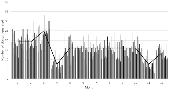
Fig. 1. Number of stands created per month in 30 repetitions (line: statistical average).
The amount of available feedstock varied between repetitions (Fig. 2). The average of the variation was –1.45%, indicating some error that needs to be compensated. The highest available amount of the feedstock was 11% higher than the statistical average. The lowest availability was 22% lower than the statistical amount.
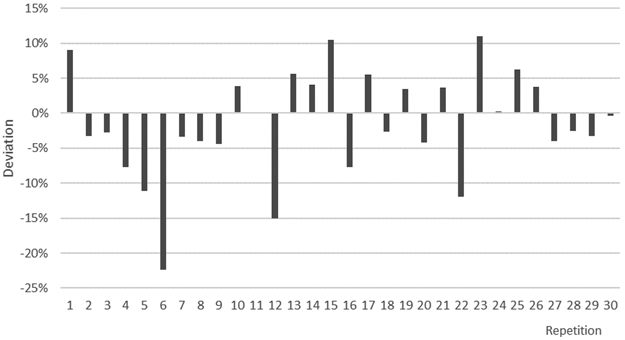
Fig. 2. Deviation of simulated biomass harvest volumes per simulation repetitions from the annual average of the total stand population.
The distance from the selected stands to the demand point varied yearly (Fig. 3). The average of all points was 75.5 km and the average of the selected points was 75.0 km. The highest average of routes in one repetition was 78.8 km and the lowest was 72.3 km.
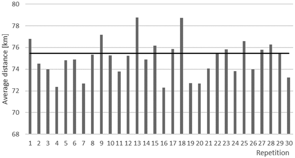
Fig. 3. Averages of simulated transport distances per simulation repetition (bars) and the average distance from all stands to the demand point (line).
3.2 Weather data validation
Precipitation was taken from Mikkeli weather data, and the factors needed for the drying models (Eq. 4 and Eq. 5) are from literature. They were assumed to correspond to the biomass storage. Evaporation was estimated by using Eq. 7 with a pan coefficient and required validation. The values were estimated with weather data from a weather station in Mikkeli (FMI 2011) in 2011. The elevation was set to 1 meter and the latitude to N60°.
Fig. 4 presents the monthly evaporation rates. It is apparent that no measurements have taken place during the colder months, as the values are zero between December and April. A dashed line represents Eq. 9. This may be incorrect, as the weather often deviates from the annual average, as for example happens with the evaporation estimation with Eq. 7, in which there is an unusually high value in July. The same effect can be seen from measured data. Eq. 7 also gives negative values during colder months, but this value should be zero, as the temperature is below zero and the evaporation is negligible.
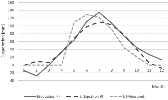
Fig. 4. Estimated evaporations and measured evaporation from the Mikkeli weather station. Equation 7: Simplified Penman-Monteith. Equation 9: VTT equation.
Using weather data from 2011 and estimating the moisture content for two years of forest biomass that has an initial moisture content of 45% with Eq. 4 using Coef = 0.062 and Const = 0.039 provides a corresponding uncovered pine stem storage (Raitila et al. 2015). The same estimation was done to Eq. 5 with constants a = 0.0008, b = 5, and c = 0.002 corresponding to the delimbed pine storage (Raitila et al. 2015). Both methods produce similar results for the first year (Fig. 5). During the winter, Eq. 4 is not valid (Routa et al. 2015b), as the moisture content is estimated to stay constant, which leads to a small error. Routa et al. (2015b) suggest a 5 percentage point increase for the winter time to correct the error. When using longer modeling periods, the error increases, as there is no limit to how dry the forest biomass may become. With Eq. 5, the equilibrium moisture term slows down the drying and prevents the moisture content from dropping under the equilibrium moisture value.
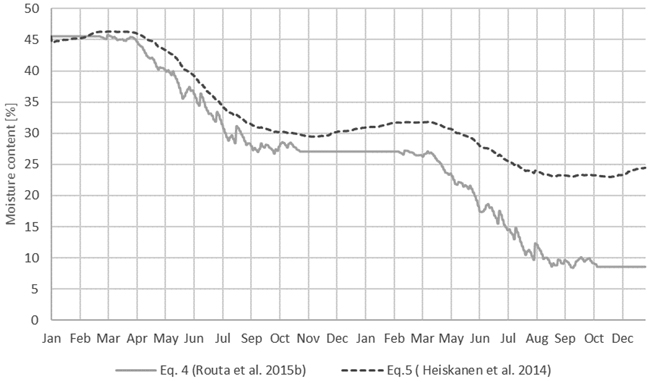
Fig. 5. Moisture content estimations with Eq. 4 (Routa et al. 2015b) and Eq. 5 (Heiskanen et al. 2014) using 2011 weather data from the Mikkeli weather station and the starting moisture 45%.
4 Discussion
The method in this study estimated forest biomass availability with annual variation. The lowest availability estimated by the method was 22% lower than the statistical amount. Despite the large difference, the value is possible to attain it in real life, although unlikely. The average difference of –1.45% in the feedstock amounts was concluded to be from the zero availability error, as some stands did not have any biomass that may be acquired from the supply point. This is a database and grid allocation specific error and shows the importance of validation. It is possible to eliminate the error by taking into account a number of zero availability points in the dataset and adding to Eq. 2 a factor of proportion of zero available points. This requires knowing the proportion of supply points with zero availability. A better option is to edit the database by removing all zero availability points beforehand.
Allocating points in the grid and selecting random points annually produced variation in the transportation distances. This indicates that the allocation of points is stochastic and suited for multi-year simulations. Having a stand allocated to the centroids of the grid is one possible allocation method for the locations. If the real stand locations of the supply area are known, these locations can be used instead of the centroid of the grid. This is possible by using forest resource information that includes the locations of the stands or by having an enterprise provide the locations of stands that are in their supply area. Having real locations of stands in the model gives more realistic roadside allocations, and if the information includes the area of the stand, it may be used as a factor for allocating initial supply amounts from the forest inventory. The method to increase the availability of one stand would still utilize Eq. 2.
A difference between the moisture estimation equations is evident. Eq. 4 seems better suited for shorter storage times, as longer storage can lead to negative moisture contents, which is not possible in real life. Eq. 4 also shows more variation on a daily scale, which is beneficial for the simulations of short storing times. If the storing time is assumed to be years, Eq. 5 would be more suitable, as the daily changes are not as relevant. As this study does not have the real storage time and cannot therefore compare the results between different moisture content estimations, the validity of the models cannot be proven. However, Raitila et al. (2015) compared both moisture content estimations with measured validation results from three validation storages and found that both estimation methods rendered good results with a variation of 0.4 to 3.2 percentage points for Eq. 4 and 0.2 to 2.8 percentage points for Eq. 5. It is important to notice that in both cases, the constants and coefficients employed affected the results greatly, and obtaining corresponding values for the simulation situation may be challenging.
The allocation method presented in this paper was capable of producing harvested stands and the required quantity of annual feedstock availability with variance, both in the location and quantity of feedstock. Forest operations may be included in the model with machinery properties and productivity. If this is done, it is important to have the stands’ feedstock amounts correspond to real life stands. The method calls for regional data and, depending on the data, some adjustment is needed, but the allocation of the stands and available feedstock may also be carried out with reasonable accuracy by the presented method.
As the simulation model imitates real-life operations, it is preferable to use real-life data, such as measured or enterprise operative data. Furthermore, if the simulation is of a theoretical situation real world data does not exist, which necessitates the use of estimated data. This forces to estimate the data. This should be done by using statistically valid data and processing the data for the simulation model as closely as possible to the real-life equivalent. For forest biomass, the supply needs to be scattered temporally and spatially with the correct availability of harvesting stands. The presented data preparation method allocates the harvested stands to the supply area, producing a valid supply network that includes variation of the feedstock amount and locations of the points.
The allocation of the supply points by using a method including stochastical elements allows the representation of the real-life annual variation of the harvested forest stands. This enables conducting a study for multiple years and further allowing the inclusion of long-time planning, yearly variations of feedstock, and annual transportation cost variations. Taking into account the uncertainty of feedstock availability and demand requirements, for example with storage terminals, requires multiple years because high storage levels change annually. Sahoo and Mani (2015) have conducted a multi-year biomass supply chain study using Miscanthus crop as feedstock. The annual feedstock availability was varied based on statistics, and the locations were kept the same. This was possible as the supply locations do not change in agriculture as much as in forestry.
Modeling every tree in the stand, as in the model by Ziesak et al. (2004), led to a need for considerable computing power. Using this method can be justified if the focus of the study is on harvesting and other forest operations. Studies focusing on the end of the supply chain may be more abstract, such as those conducted by Aalto et al. (2018) and Väätäinen et al. (2005). Methods described in this paper allow simplifying feedstock availability for wider supply chain simulation studies while maintaining the realistic locations and temporal variation of the supply. There are many advantages to including spatial analysis compared to random allocation.
Eriksson et al. (2017) have used random locations inside a circle to generate forest stands around a demand location. Although this gives varying transportation distances, it does not take local variables into account, such as the amount of feedstock at the location or harvesting time allocations due to weather variables. In addition, limiting factors for supply areas are not taken into account (e.g. water bodies or urban areas). Using GIS allows allocation of the stands to more realistic locations and even in real locations if this data is available. In addition, the availability can be restricted based on road limitations, and distances may be calculated based on different route selections (shortest, fastest, limited access, etc.). If real locations are used, it is possible to limit the availability based on extraction distances as the distance from the stand to the nearest road.
The case that this paper examines uses a database to acquire theoretical feedstock availability. The method can be used for different availability information to distribute availability temporally and spatially. This availability information can be based on previous supply information or the statistical distribution of supply. In addition to this, the supply area may vary, as the total number of supply points (Eq. 2: Nsp) and the total feedstock amount (Eq. 2: Vsp,i ) change when this area is changed. The same effect is accomplished if some places are set to inaccessible and removed from the availability of feedstock. The flexibility and scenario-based nature of the simulation study method allow many different usages for the method. A round supply area is often optimal, but the road network structure and inaccessible locations may change this.
As the moisture content of the feedstock affects the amount of stored energy of the biomass, the moisture content change should be taken into account when studying the supply system. There are different possible methods for this, but they may increase the computational power requirements or do not take local weather variations into account. Windisch et al. (2015) have used drying curves, which demand less computational power than estimation equations but do not consider local weather variations. The method may be used with fewer values, using more estimations, but this leads to less accurate results, making the simulation model less valid.
Using weather station data and equations to estimate the moisture content, the effect of weather can be accounted for by changing the quality of the forest biomass. These results can be acquired with a different amount of available data by using equations to estimate values that are not often measured or are complicated to calculate. The accuracy of the results and the model decrease with estimations, and therefore, it is recommendable to avoid unnecessary estimations. The estimations should be validated and verified case-specifically, as the level of abstraction and the purpose of the simulation model affect the importance of the data preparation.
The addition of weather-based moisture changes to the model enables studying alternative decision-making in the delivery strategies in cases where the moisture is known. The model may focus on high quality feedstock during the high demand season and leave low quality feedstock at supply locations during the low demand season. This has been done by Eriksson et al. (2017) with moisture estimation equations, although the implication of the equations in the model are not presented in detail. Eriksson et al. (2017) state that a weather-driven approach enables the model to account for variations between different years and supply points. When this is included with supply location allocation, the model has more real-life conditions for the feedstock supply and generates more realistic scenarios for the study.
The supply point allocation method presented in this paper allows distributing theoretical annual availability spatially and temporally to the selected supply area. GIS enables considering location specific restrictions and obtaining transportation distances based on the road network. The method generates a more realistic supply network than random allocation. The possibility to modify the supply area offers the opportunity to take spatial restrictions of feedstock availability into account. Moisture equations take quality changes into account, although implementing them into the model is challenging and lowers its validity. Methods described in this paper can be used for multi-year biomass supply chain simulations, which require annual variations of supply locations, feedstock availability, and quality changes.
Acknowledgements
This study is part of the project Improvement of forest chip quality and supply chain performance by means of a continuous quality measurement system (JATKUMO). Support from the European Unions Structural Funds have made it possible to conduct JATKUMO and this study.
References
Aalto M., Korpinen OJ., Loukola J., Ranta T. (2018). Achieving a smooth flow of fuel deliveries by truck to an urban biomass power plant in Helsinki, Finland – an agent-based simulation approach. International Journal of Forest Engineering 29(1):21–30. https://doi.org/10.1080/14942119.2018.1403809.
Alakangas E., Hurskainen M., Laatikainen-Luntama J., Korhonen J. (2016). Properties of indigenous fuels in Finland. VTT Technology 272. VTT Technical Research Centre of Finland, Espoo. 222 p. ISBN 978-951-38-8456-7.
Allen J., Browne M., Hunter A., Boyd J., Palmer H. (1998a). Logistics management and costs of biomass fuel supply. International Journal of Physical Distribution & Logistics Management 28(6): 463–477. https://doi.org/10.1108/09600039810245120.
Allen R.G., Pereira L.S., Raes D., Smith M. (1998b). Crop evapotranspiration (guidelines for computing crop water requirements). FAO Irrigation and drainage paper 56. Food and Agriculture Organization, Rome. 254 p.
Asikainen A. (1995). Discrete-event simulation of mechanized wood-harvesting systems. D.Sc. thesis, University of Joensuu, Joensuu. 86 p.
Awadalla H.S.F., El-Dib A.F., Mohamad M.A., Reuss M., Hussein H.M.S. (2004). Mathematical modelling and experimental verification of wood drying process. Energy Conversion and Management 45(2): 197–207. https://doi.org/10.1016/S0196-8904(03)00146-8.
Datta P., Dees M., Elbersen B., Staritsky I. (2017). The data base of biomass cost supply data for EU 28, Western Balkan Countries, Moldova, Turkey and Ukraine. Project Report. Chair of Remote Sensing and Landscape Information Systems, Institute of Forest Sciences, University of Freiburg, Germany. 25 p.
Demirbas M.F., Balat M., Balat H. (2009). Potential contribution of biomass to the sustainable energy development. Energy Conversion and Management 50(7): 1746–1760. https://doi.org/10.1016/j.enconman.2009.03.013.
Erber G., Kanzian C., Stampfer K. (2012). Predicting moisture content in a pine logwood pile for energy purposes. Silva Fennica 46(4): 555–567. https://doi.org/10.14214/sf.910.
Eriksson A., Eliasson L., Hansson P.A., Jirjis R. (2014a). Effects of supply chain strategy on stump fuel cost: a simulation approach. International Journal of Forestry Research 2014 article 984395. 11 p. https://doi.org/10.1155/2014/984395.
Eriksson A., Eliasson L., Jirjis R. (2014b). Simulation-based evaluation of supply chains for stump fuel. International Journal of Forest Engineering 25(1): 23–36. https://doi.org/10.1080/14942119.2014.892293.
Eriksson A., Eliasson L., Sikanen L., Hansson P.A., Jirjis R. (2017). Evaluation of delivery strategies for forest fuels applying a model for Weather-driven Analysis of Forest Fuel Systems (WAFFS). Applied energy 188: 420–430. https://doi.org/10.1016/j.apenergy.2016.12.018.
FMI (2011) Weather and sea, download observations. https://en.ilmatieteenlaitos.fi/download-observations/. Finnish Meteorological Institute. [Cited 16 Oct 2018].
Gallego-Elvira B., Baille A., Martin-Gorriz B., Maestre-Valero J.F., Martinez-Alvarez V. (2012). Evaluation of evaporation estimation methods for a covered reservoir in a semi-arid climate (south-eastern Spain). Journal of hydrology 458: 59–67. https://doi.org/10.1016/j.jhydrol.2012.06.035.
Gigler J.K., van Loon W.K., Seres I., Meerdink G., Coumans W.J. (2000). PH—postharvest technology: drying characteristics of willow chips and stems. Journal of Agricultural Engineering Research 77(4): 391–400. https://doi.org/10.1006/jaer.2000.0590.
Heiskanen VP., Raitila J., Hillebrand K. (2014). Varastokasassa olevan energiapuun kosteuden muutoksen mallintaminen. [Modeling of moisture change in energy wood in a storage]. Report VTT-R-08637-13. 26+1 p. [In Finnish].
Holopainen M., Vastaranta M., Rasinmäki J., Kalliovirta J., Mäkinen A., Haapanen R., Melkas T., Yu X., Hyyppä J. (2010). Uncertainty in timber assortment estimates predicted from forest inventory data. European Journal of Forest Research 129(6): 1131–1142. https://doi.org/10.1007/s10342-010-0401-4.
Islam M.N., Pukkala T., Kurttila M., Mehtätalo L., Heinonen T. (2012). Effects of forest inventory errors on the area and spatial layout of harvest blocks. European journal of forest research 131(6): 1943–1955. https://doi.org/10.1007/s10342-012-0645-2.
Kanzian C., Kühmaier M., Erber G. (2016). Effects of moisture content on supply costs and CO2 emissions for an optimized energy wood supply network. Croatian Journal of Forest Engineering: Journal for Theory and Application of Forestry Engineering 37(1): 51–60.
Kim D.W., Murphy G. (2013). Forecasting air-drying rates of small Douglas-fir and hybrid poplar stacked logs in Oregon, USA. International Journal of Forest Engineering 24(2): 137–147. https://doi.org/10.1080/14942119.2013.798132.
Liang T., Khan M.A., Meng Q. (1996). Spatial and temporal effects in drying biomass for energy. Biomass and Bioenergy 10(5–6): 353–360. https://doi.org/10.1016/0961-9534(95)00112-3.
Linacre E.T. (1977). A simple formula for estimating evaporation rates in various climates, using temperature data alone. Agricultural meteorology 18(6): 409–424. https://doi.org/10.1016/0002-1571(77)90007-3.
LUKE (2018a). Biomass-atlas. https://www.luke.fi/biomassa-atlas/en/. Natural Resources Institute Finland (Luke). [Cited 16 Oct 2018].
LUKE (2018b). Industrial roundwood removals and labour force – harvesting volumes of energy wood per month. http://statdb.luke.fi/PXWeb/pxweb/en/LUKE/. Natural Resources Institute Finland (Luke). [Cited 16 Oct 2018].
MacDonald A.J. (2007). Estimated costs for harvesting, comminuting, and transporting beetle-killed pine in the Quesnel/Nazko area of central British Columbia. In: Proceedings of the International Mountain Logging and 13th Pacific Northwest Skyline Symposium, Corvallis, OR. p. 208–214.
Mobini M., Sowlati T., Sokhansanj S. (2011). Forest biomass supply logistics for a power plant using the discrete-event simulation approach. Applied energy 88(4): 1241–1250. https://doi.org/10.1016/j.apenergy.2010.10.016.
Monteith J.L. (1981). Evaporation and surface temperature. Quarterly Journal of the Royal Meteorological Society 107(451): 1–27. https://doi.org/10.1002/qj.49710745102.
Murphy G., Kent T., Kofman P.D. (2012). Modeling air drying of Sitka spruce (Picea sitchensis) biomass in off-forest storage yards in Ireland. Forest Products Journal 62(6): 443–449. https://doi.org/10.13073/FPJ-D-12-00096.1.
Nabuurs G.J., Pussinen A., Van Brusselen J., Schelhaas M.J. (2007). Future harvesting pressure on European forests. European Journal of Forest Research 126(3): 391–400. https://doi.org/10.1007/s10342-006-0158-y.
OpenStreetMap contributors (2018). Planet dump retrieved from https://planet.osm.org; https://www.openstreetmap.org.
Plumb O.A., Spolek G.A., Olmstead B.A. (1985). Heat and mass transfer in wood during drying. International Journal of Heat and Mass Transfer 28(9): 1669–1678. https://doi.org/10.1016/0017-9310(85)90141-3.
Raitila J., Heiskanen V.P., Routa J., Kolström M., Sikanen L. (2015). Comparison of moisture prediction models for stacked fuelwood. BioEnergy Research 8(4): 1896–1905. https://doi.org/10.1007/s12155-015-9645-7.
Rentizelas A.A., Tolis A.J., Tatsiopoulos I.P. (2009). Logistics issues of biomass: the storage problem and the multi-biomass supply chain. Renewable and sustainable energy reviews 13(4): 887–894. https://doi.org/10.1016/j.rser.2008.01.003.
Routa J., Kolström M., Ruotsalainen J., Sikanen L. (2015a). Precision measurement of forest harvesting residue moisture change and dry matter losses by constant weight monitoring. International Journal of Forest Engineering 26(1): 71–83. https://doi.org/10.1080/14942119.2015.1012900.
Routa J., Kolström M., Ruotsalainen J., Sikanen L. (2015b). Validation of prediction models for estimating the moisture content of small diameter stem wood. Croatian Journal of Forest Engineering: Journal for Theory and Application of Forestry Engineering 36(2): 283–291.
Sahoo K., Mani S. (2015). GIS based discrete event modeling and simulation of biomass supply chain. In: 2015 Winter Simulation Conference (WSC). p. 967–978. https://doi.org/10.1109/WSC.2015.7408225.
Salama M.A., Yousef K.M., Mostafa A.Z. (2015). Simple equation for estimating actual evapotranspiration using heat units for wheat in arid regions. Journal of Radiation Research and Applied Sciences 8(3): 418–427. https://doi.org/10.1016/j.jrras.2015.03.002.
Sikanen L., Röser D., Anttila P., Prinz R. (2013). Forecasting algorithm for natural drying of energy wood in forest storages. Forest Energy Observer. Study Report 27.
SYKE (2011). Hydrologiset kuukausitilastot. [Hydrological monthly statistics]. http://wwwi3.ymparisto.fi/i3/paasivu/fin/etusivu/etusivu.htm. Finnish Environment Institute (SYKE). [Cited 16 Oct 2018].
Väätäinen K., Asikainen A., Eronen J. (2005). Improving the logistics of biofuel reception at the power plant of Kuopio city. International Journal of Forest Engineering 16(1): 51–64. https://doi.org/10.1080/14942119.2005.10702507.
Wasajja H., Chowdhury S.D. (2017). Evaluation of advanced biomass technologies for rural energy supply. In: 2017 IEEE AFRICON. p. 1272–1276. https://doi.org/10.1109/AFRCON.2017.8095665.
Windisch J., Väätäinen K., Anttila P., Nivala M., Laitila J., Asikainen A., Sikanen L. (2015). Discrete-event simulation of an information-based raw material allocation process for increasing the efficiency of an energy wood supply chain. Applied energy 149: 315–325. https://doi.org/10.1016/j.apenergy.2015.03.122.
Ziesak M., Bruchner A.K., Hemm M. (2004). Simulation technique for modelling the production chain in forestry. European Journal of Forest Research 123(3): 239–244. https://doi.org/10.1007/s10342-004-0028-4.
Total of 43 references.
