Jaakko Repola  ,
Juha Heikkinen,
Jari Lindblad
,
Juha Heikkinen,
Jari Lindblad
Pulpwood green density prediction models and sampling-based calibration
Repola J., Heikkinen J., Lindblad J. (2021). Pulpwood green density prediction models and sampling-based calibration. Silva Fennica vol. 55 no. 4 article id 10539. https://doi.org/10.14214/sf.10539
Highlights
- The developed models provided a realistic description of the observed seasonal variation in pulpwood green density
- The model predictions were more reliable than those obtained with current practices.
Abstract
Pulpwood arriving at the mills is mainly measured by weighing. In the loading phase of forwarding and trucking, timber is weighed using scales mounted in the grapple loader. The measured weight of timber is converted into volume using a conversion factor defined as green density (kg m–3). At the mill, the green density factor is determined by sampling measurements, while in connection with weighing with grapple-mounted scales during transportation, fixed green density factors are used. In this study, we developed predictive regression models for the green density of pulpwood. The models were constructed separately by pulpwood assortments: pine (contains mainly Pinus sylvestris L); spruce (mainly Picea abies (L.) Karst.); decayed spruce; birch (mainly Betula pubescens Ehrh. and Betula pendula Roth); and aspen (mainly Populus tremula L.). Study material was composed of the sampling-based measurements at the mills between 2013–2019. The models were specified as linear mixed models with both fixed and random parameters. The fixed effect produced the expected value of green density as a function of delivery week, storage time, and meteorological conditions during storage. The random effects allowed the model calibration by utilizing the previous sampling weight measurements. The model validation showed that the model predictions faithfully reproduced the observed seasonal variation in green density. They were more reliable than those obtained with the current practices. Even the uncalibrated (fixed) predictions had lower relative root mean squared prediction errors than those obtained with the current practices.
Keywords
pulpwood;
conversion factor;
green density
-
Repola,
Natural Resources Institute Finland (Luke), Natural resources, Ounasjoentie 6, 96200 Rovaniemi, Finland
E-mail
jaakko.repola@luke.fi
- Heikkinen, Natural Resources Institute Finland (Luke), Production systems, Yliopistokatu 6, FI-80100 Joensuu, Finland E-mail juha.heikkinen@luke.fi
- Lindblad, Natural Resources Institute Finland (Luke), Natural resources, Latokartanonkaari 9, 00790 Helsinki, Finland E-mail jari.lindblad@luke.fi
Received 8 March 2021 Accepted 12 August 2021 Published 19 August 2021
Views 58910
Available at https://doi.org/10.14214/sf.10539 | Download PDF

Supplementary Files
1 Introduction
In Finland, timber measurement by harvester-based devices is the most common method of determining timber purchase prices in standing sales. Despite this, timber is measured at the mill to determine the amounts of timber exchanged by companies and the amount of incoming timber. In addition, timber can be measured in connection with forest hauling or long-distance transportation, or rarely, at the roadside storage. It is common that the same parcel of timber is measured more than once and for different needs of measurement information during the procurement chain.
Nowadays, the pulpwood arriving at the mills is mainly measured by weighing. The share of weighing in the mill measurement of pulpwood was about 95 percent in 2019 (Melkas 2020). Weighing has strongly superseded other measurement methods and technologies at the mills in recent ten years. Concerning delivery sales, loader-mounted weighing has replaced the measurement of pulpwood in stacks at the roadside. About 3.0 million cubic meters of sawlogs and pulpwood were measured by loader scale measurement in 2019. In delivery sales, the share of loader scale measurement was 45 percent (2.8 million m³) (Melkas 2020).
As mentioned, timber measurement methods based on weighing have become common during the 2010s. The main reason for this development has been the flexible integration of weighing with forest hauling, transportation and processes at the mills. Weighing is a cost-effective and fast method to measure large quantities of pulpwood arriving at the mills. Measurement by weighing also has the advantage of being based on robust and reliable measurement technology (Sikanen et al. 1992; Heikkilä et al. 2004).
The weight of timber can be used directly as the basis for transport contracting fees. However, for other needs of measurement information, such as determining purchase prices or logging entrepreneurs’ fees, solid volume is the final quantity of interest. The measured weight of the timber must then be converted into volume using green density (kg m–3), a conversion factor defined as the relation between weight and solid volume, including bark.
Concerning commonly used weight measurement, the methods can be divided into two main parts: sampling-based weight measurement using stationary vehicle scales or unloading devices at the mills and weighing with grapple-mounted scales during transportation. The methods do not differ only in terms of the location of measurement operations and the measurement devices used. The essential difference between the methods is also related to the conversion factors between volumes and weights. The resultant weight determined by grapple scales can be converted into volume according to fixed green density factors by timber assortments. Regional green density factors by timber assortments, month, and freshness class have been issued on a regulatory basis (Natural Resources Institute Finland 2017). Instead, as “method” indicates, the green density factor is determined at the mill by sampling and objective sample measurements. At a practical level, differences in the values of the conversion factors between these measurement methods are not appropriate and may in some cases lead to ambiguities.
The sampling-based weight measurement method consists of five stages: weighing the entire timber arriving at the mill; selecting the sample bundles of timber; measuring the green density of the sample bundles; calculating and maintaining the green density factors; and determining the solid volumes of timber by using sampling-based conversion factors.
Sampling-based weighing is currently mill-specific. In most cases, the population for sampling is formed according to timber assortments so that several timber suppliers belong to the same sampling population. The sample bundles are selected using random sampling. The actual sampling percentage for the main timber assortments at the mill is typically 2–4% of the total incoming pulpwood. For the timber assortments with a relatively low total volume, the sampling percentage can be as high as 10–15%.
The green density of the individual sample bundle is determined by measuring the weight and solid volume of the timber. The solid volume is generally measured by hydrostatic measurement through immersion in water and weighing. The current conversion factor (green density) is determined as a trimmed moving average of the sample measurements obtained during the last 5–7 days. For example, the green density factor may be computed as the average of the measured green density of five bundles selected from the last seven sample bundles by discarding the lowest and highest observations. The current conversion factor is a constant value, and it is applied to all arriving pulpwood loads. It is obvious that the calculation of the conversion factor as a trimmed moving average is sensitive to a random variation of green density observations.
The green density of pulpwood, or equivalently, moisture content, varies due to e.g. different storage conditions such as duration, weather conditions, season, etc. The current practice, including both sampling and fixed conversion factors, does not take these factors explicitly into account, which may lead to an unrealistic volume estimate e.g. for a pulpwood parcel with low moisture content caused by long storage. The need for improvements in the current system has been widely recognized, meaning the factors known to affect the moisture content can be taken into account, and more reliable green density values can be attached to each arriving pulpwood load. One approach is to construct a regression model for predicting green density based on variables describing the main storage conditions (Hultnäs et al. 2012; Lindblad and Repola 2019). Hultnäs et al. (2012) developed the model for the green density of Norway spruce pulpwood by using density data from earlier years for a certain mill and meteorological data from its wood supply area. Lindblad and Repola (2019) presented linear mixed models for the green density of pine and birch pulpwood based on the date of measurement at the mill and storage time.
The conclusion of the previous studies (Hultnäs et al. 2012; Lindblad and Repola 2019) was that the developed models enabled the determination of general green density values, but not the determination of green density for practical purposes. Lindblad and Repola (2019) emphasized that meteorological factors should also be included in the model, because weather conditions have a notable effect on wood drying during storage and cause significant variation between regions and years. Lindblad and Repola (2019) showed that green density values could change in a short period, especially in the spring, when there were marked systematic differences between predictions based on fixed effect only and the modeling data’s observed mean trend. The risk of such systematic deviations will also be present in the application phase when the models are applied to new data of upcoming years. An essential requirement of an operational green density model is therefore that it can be calibrated flexibly with new observations (sample weight measurements) in adequate intervals. Lindblad and Repola (2019) constructed the model with a random year effect, enabling year-level calibration. For practical needs, the year-level calibration has proven too inexact, and week-level calibration has been identified as a potentially reasonable compromise between temporal accuracy and sampling requirements. As measurements from one week’s incoming pulpwood may not be sufficient for reliable calibration, the model should be formulated so that also the previous weeks’ measurements can be utilized.
The aim of this study was to develop tools that could be utilized in the sampling-based weight measurement to estimate the green density (conversion factor) of pulpwood arriving at pulp mills. Predictive models were constructed for the dependence of green density (kg m–3) of pulpwood on different storage variables (duration, season, weather conditions). They were formulated as linear mixed models, where the fixed part of the model gives the expected greed density as a function of the storage variables and the random part was specified in such way that the predictions can be flexibly calibrated within a short timespan to new pulpwood parcels by utilizing the most recent sample measurements. The structure of the random part was motivated by the need to control the precision of the future predictions of random components in the operational application by setting weekly sample size requirements to calibration data.
2 Materials and methods
2.1 Materials
The study material was composed of the sampling-based measurements of pulpwood (green density, kg m–3) that were carried out in paper and pulp mills (Metsä Fibre Ltd, UPM-Kymmene Ltd, Stora Enso Ltd) between 2013–2019 in Finland. The mills (N = 17) were located in different parts of Finland, and their timber supply areas covered almost the entire country, composing a significant share of pulpwood flow in Finland (Fig. 1). The total number of mills using the weight sampling method was 21, which also indicates the good coverage and representativeness of the research data in this respect.
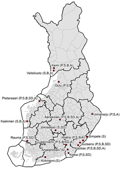
Fig. 1. Locations of the paper and pulp mills from which sample-based measurements were included in the green density prediction study material (P = pine, S = spruce, B = birch, SD = decayed spruce, A = aspen).
The study material was restricted to those observations in which green density measurements were coupled with information on timber assortment, the date of arrival at the mills, the date of harvesting, and the origin of timber, i.e. the location of a stand marked for harvesting. A total of 53 775 sample-based observations fulfilled this criterion. The data were distributed between the main pulpwood assortments so that 38% was pine (contains mainly Pinus sylvestris L.), 32% birch (mainly Betula pubescens Ehrh. and Betula pendula Roth), 20% spruce (mainly Picea abies (L.) Karst.), 6% decayed spruce, and 4% aspen (mainly Populus tremula L.) (Table 1). There was a lot of variation in storage time, and the observations were distributed in two groups of almost equal size: those that were stored less than one month (48.7%), and those that were stored longer (51.3%). The average storage time varied by pulpwood assortments from 39 to 70 days, but long storage times exceeding one year were also found for all assortments (Table 2).
| Table 1. The number of observations by pulpwood assortments in the green density prediction study material. | ||||||||
| Pulpwood assortment | Total | Year | ||||||
| 2013 | 2014 | 2015 | 2016 | 2017 | 2018 | 2019 | ||
| Pine 1) | 20 299 | 3421 | 2488 | 4677 | 3699 | 2456 | 1867 | 1691 |
| Spruce 2) | 10 769 | 1120 | 1072 | 1344 | 1706 | 2015 | 1955 | 1557 |
| Spruce, decayed 3) | 2991 | 221 | 238 | 304 | 447 | 789 | 538 | 454 |
| Birch 4) | 17 423 | 2854 | 2455 | 3111 | 3027 | 2446 | 1852 | 1678 |
| Aspen 5) | 2293 | 281 | 222 | 215 | 365 | 522 | 385 | 303 |
| 1) Contain mainly Scots Pine (Pinus sylvestris); 2), 3) mainly Norway spruce (Picea abies); 4) mainly downy birch (Betula pubescens) or/and silver birch (Betula pendula); 5) mainly aspen (Populus tremula). | ||||||||
| Table 2. Green density (kg m–3) values and storage time of green density prediction study material by pulpwood assortments. | |||||||
| Pulpwood assortment | Number of observations | Green density, kg m–3 | Storage time, days | ||||
| Mean | Std | Median | Mean | Std | Median | ||
| Pine | 20 299 | 878.9 | 71.0 | 892 | 70 | 83 | 40 |
| Spruce | 10 769 | 845.7 | 64.3 | 854 | 38 | 48 | 21 |
| Spruce, decayed | 2991 | 731.6 | 56.4 | 732 | 43 | 56 | 26 |
| Birch | 17 423 | 868.3 | 65.9 | 881 | 70 | 79 | 40 |
| Aspen | 2293 | 804.4 | 60.2 | 809 | 50 | 57 | 29 |
The Finnish Meteorological Institute (FMI) provides gridded weather data covering the whole of Finland. This dataset consists of quantities measured at weather observation stations and interpolated into a 10-km × 10-km grid by kriging (Venäläinen and Heikinheimo 2002). Interpolations to a 1-km × 1-km grid have also been available in recent years (Aalto et al. 2013). The meteorological data used in this study were stored as grid square values in a database. The data were divided into two different parts according to the grid resolution and available weather observations. The 10-km × 10-km grid data from the beginning of 2012 to November 2016 consisted of observations of minimum, maximum, and average temperature (°C), rainfall (mm), global radiation (W m–2), and air pressure (hPa) at the day level. In addition to the previous variables, the 1-km × 1-km grid data from November 2016 to the end of 2019 included maximum and average wind speed (m s–1), average wind direction, relative air humidity (%) (min., max., avg.), potential evaporation (mm), and snow depth (cm).
The geographical origin of individual timber lots in the study material was known at municipality level. The meteorological data for each municipality was generated by using the location of the geographical center of the municipality and extracting the interpolated weather observations from the nearest grid square. The resulting meteorological data consisted of daily weather observations from 310 municipalities in 2012–2019. The year 2012 was included in the data, because a significant part of the timber arriving at the mills, especially at the beginning of 2013, was harvested in 2012.
Weather-based variables related to the storage period of the individual timber lots in the research material were calculated using the municipality-specific meteorological data. The calculation was carried out using daily weather observations between the dates of harvesting and arrival at the mill. All the variables were constructed as cumulative sums or averages of different precipitation and temperature observations.
2.2 Model approaches
Regression models for green density (kg m–3) were constructed separately by pulpwood assortments: pine, spruce, decayed spruce, birch, and aspen. The dependent variable, the green density of pulpwood (kg m–3), was obtained from the sampling-based weight measurements at the mills. The compiled models had two main requirements. First, the models needed to account for the main factors affecting wood drying during storage and produce the green density prediction for each arriving pulpwood load at mills when the required input variables were available. This required the models to be based only on the variables that were commonly available, or which could be derived easily and reliably from a database. It also needed to be implementable in an operational pulpwood receiving system. This last restriction ruled out non-parametric regression models in practice. Second, the model structure had to enable the calibration of predictions with real-time sampling-based weight measurements to track the current level of green density values at the national level. The material gathered in 2013–2018 was used to construct the models, and the material from 2019 was saved for model validation and the demonstration of real-time calibration with new sample weight measurements.
Linear mixed models with fixed and random effects were applied, because they offer a flexible framework for addressing correlation structures in model residuals and support calibration (Parresol 1999; McCulloch and Searle 2001). The models were constructed separately for the pulpwood assortments of pine, spruce, decayed spruce, birch, and aspen. The basic models (MODELS 1) allow for nationwide calibration only. Their general form is:
![]()
where i, j, and k refer to year, week number, and pulpwood parcel respectively, GDijk is the response variable (green density of pulpwood, kg m–3), β is a vector of fixed effects parameters, Xijk is the vector of independent variables indicating delivery date, storage time, and weather conditions during the storage, wij is a random week effect, and eijk is the model residual. The covariance structure of the successive weeks was assumed to follow the first-order autoregressive (AR-1) structure with unknown correlation parameter ρ to be estimated as part of model fitting. The residuals (eijk) were assumed to be mutually uncorrelated, and also uncorrelated with the random effects (wij). Both wij‘s and eijk‘s were assumed to be Gaussian with a mean of zero. Constant variance ![]() was assumed for the week effects, but a similar assumption did not appear reasonable for the residuals, the variability of which appeared to depend on both the season of the delivery and the storage time. Hence, the residual variances
was assumed for the week effects, but a similar assumption did not appear reasonable for the residuals, the variability of which appeared to depend on both the season of the delivery and the storage time. Hence, the residual variances ![]() were estimated separately in four groups, g = 1, ... 4, delineated by delivery month (January–May vs. June–December) and storage time (up to one month vs. longer).
were estimated separately in four groups, g = 1, ... 4, delineated by delivery month (January–May vs. June–December) and storage time (up to one month vs. longer).
To enable regional calibration, we constructed a second set of models (MODELS 2):
![]()
with region-specific week effect wijr, where r refers to one of the sub-areas shown in Fig. 2. Separate variance and correlation parameters, ![]() and ρr, for the week effects were estimated for each region. Otherwise, MODELS 2 were similar to MODELS 1 with the same covariates. But the β parameters were estimated separately for the two types of models, because the estimates depend on the assumed covariance structure. MODELS 2 were fitted to the main pulpwood assortments (pine, spruce, birch), which had a sufficient number of observations for estimating the parameters of the random part by sub-areas.
and ρr, for the week effects were estimated for each region. Otherwise, MODELS 2 were similar to MODELS 1 with the same covariates. But the β parameters were estimated separately for the two types of models, because the estimates depend on the assumed covariance structure. MODELS 2 were fitted to the main pulpwood assortments (pine, spruce, birch), which had a sufficient number of observations for estimating the parameters of the random part by sub-areas.
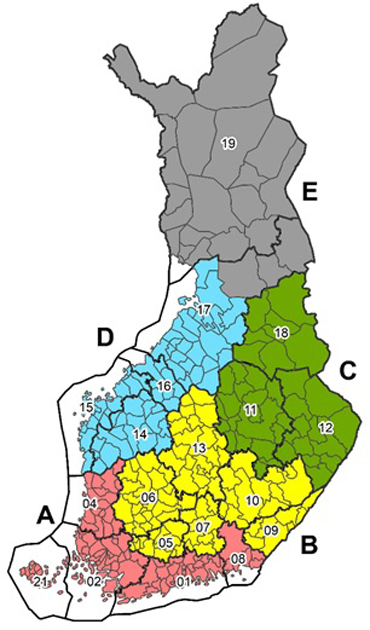
Fig. 2. Sub-areas (A–E) for the regional calibration used in green density MODELS 2.
There was constructed also complementary models (MODELS 3 and 4) for pulpwood parcels in which only delivery date and place are available. MODELS 3 were based only delivery date, and MODELS 4 also on location of the mill by using the sub-areas shown in Fig. 2. The random part of MODELS 3 and 4 were similar to MODELS 1.
The maximum likelihood (ML) method in the MIXED procedure of SAS (SAS Institute Inc. 1999) was used in the estimation of the models. Model residuals were visually inspected against the independent variables, and the detected lack of fit was addressed by adding new variables or making variable transformations. The selection of the independent variables was based on the detected relation between independent and dependent variables and residuals inspections in the study material, and only variables with a significance of t-value < 0.05 were accepted in the model. The results of the previous studies were also utilized to identify the potential transformations of the original variables (Hultnäs et al. 2012; Lindblad and Repola 2019).
2.3 Performance assessment
Predictions constructed for the 2019 test data using their observed values of predictor variables were compared to the measured green density values. Predictions were produced both by applying the fixed part of the fitted models alone, ![]() and by calibrating with the predicted week effect,
and by calibrating with the predicted week effect, ![]() The green density measurements of the past four weeks before the delivery day of parcel k were used to construct the best linear unbiased prediction
The green density measurements of the past four weeks before the delivery day of parcel k were used to construct the best linear unbiased prediction ![]() for
for ![]() (see Suppl. file S1, for details). The assessments presented here focused on the nationwide MODELS 1; the regional calibration with MODELS 2 is demonstrated for pine. The model predictions were also compared with values obtained by applying the current practices to the test data: 1) a trimmed moving average of the last seven sample measurements from the same mill, ignoring the lowest and highest observations (MOVING AVG) and 2) fixed green density factors (FGDF) by timber assortment (Natural Resources Institute Finland 2017). All four methods were compared in terms of both the parcel-level predictions and their weekly averages by calculating the relative mean squared prediction errors,
(see Suppl. file S1, for details). The assessments presented here focused on the nationwide MODELS 1; the regional calibration with MODELS 2 is demonstrated for pine. The model predictions were also compared with values obtained by applying the current practices to the test data: 1) a trimmed moving average of the last seven sample measurements from the same mill, ignoring the lowest and highest observations (MOVING AVG) and 2) fixed green density factors (FGDF) by timber assortment (Natural Resources Institute Finland 2017). All four methods were compared in terms of both the parcel-level predictions and their weekly averages by calculating the relative mean squared prediction errors,

where ![]() is the observed green density of the weekly average,
is the observed green density of the weekly average, ![]() is the corresponding value obtained by the developed models or the current practices, and n is the number of observations or weeks.
is the corresponding value obtained by the developed models or the current practices, and n is the number of observations or weeks.
3 Results
3.1 Models
The green density values of the study material showed high variation for all pulpwood assortments. Despite this, a systematic trend of seasonal variation was detected (Fig. 3). The average green density shown was highest in parcels delivered during the winter months and decreased quite steeply in the spring months (April–May), being at their lowest level in the summer months. Toward the end of the year, green density values started increasing again. This seasonal trend was described in all models using the week number of the delivery date (1–53). The week number (WEEK) was used as a continuous variable, and different power transformations (WEEK2, WEEK3) were also attempted (Table 3, Suppl. files S2, S3 and S4). In addition, all the models contained the continuous variable, which assumed non-zero values only for parcels delivered after a specific week (knot) i.e. x = max(0,WEEK – knot).
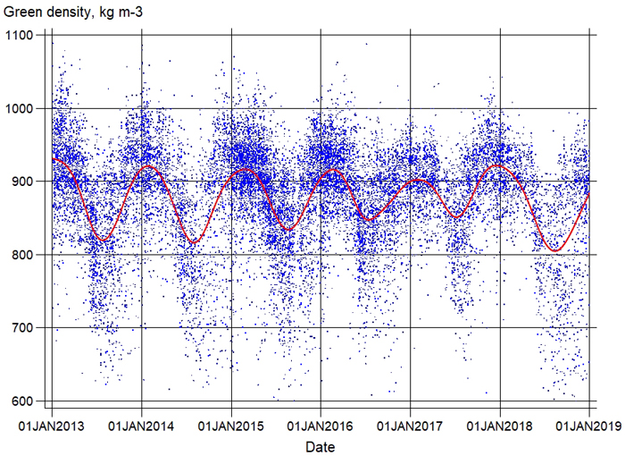
Fig. 3. Green density values of pine of the green density modeling data in 2013–2018. Red line indicates trimmed moving average.
| Table 3. Parameter estimates of models for green density (kg m–3) of the pulpwood assortments (MODELS 1). The standard error of the estimates is presented in parenthesis. | |||||
| Pine | Spruce | Spruce, decayed | Birch | Aspen | |
| Variable | Estimate | Estimate | Estimate | Estimate | Estimate |
| Intercept | 908.07 (3.753) | 865.05 (3.431) | 749.79 (6.566) | 931.56 (6.644) | 362.91 (113.98) |
| WEEK | –1.224 (0.466) | –4.078 (1.048) | |||
| WEEK>22 | 5.431 (1.176) | 2.085 (0.672) | |||
| WEEK2 | –0.061 (0.014) | 0.339 (0.068) | |||
| WEEK2>15 | 0.535 (0.098) | ||||
| WEEK2>20 | 0.194 (0.083) | ||||
| WEEK2>22 | 1.015 (0.172) | ||||
| WEEK3 | –0.0052 (0.001) | –0.01165 (0.002) | –0.0014 (0.0006) | ||
| STORAGE | –0.219 (0.043) | –0.307 (0.068) | –1.033 (0.080) | –0.733 (0.038) | –0.496 (0.092) |
| STORAGE>300 days | 0.284 (0.020) | 0.259 (0.107) | 0.245 (0.053) | 0.295 (0.021) | |
| STORAGENov-March | 0.264 (0.047) | 0.204 (0.075) | 0.686 (0.042) | ||
| STORAGEOct-Apr | 1.125 (0.073) | ||||
| STORAGEDec-March | 0.345 (0.104) | ||||
| STORAGEMay | –0.333 (0.087) | 0.445 (0.084) | |||
| STORAGEJune | –0.716 (0.094) | –1.268 (0.144) | 0.395 (0.104) | ||
| STORAGEJuly | –0.539 (0.109) | ||||
| TS | –0.157 (0.008) | –0.162 (0.015) | –0.034 (0.007) | –0.067 (0.010) | |
| TEMP | –0.532 (0.166) | –6.439 (1.189) | |||
| ln(TEMP+30) | 138.19 (33.746) | ||||
| TEMP3month | –0.791 (0.126) | –0.767 (0.290) | –0.765 (0.121) | ||
| TEMPmax20 | 0.550 (0.102) | 0.821 (0.201) | 0.433 (0.083) | ||
| ln(TEMPmax20 +1) | –4.081 (0.902) | ||||
| RAINFALL | 0.304 (0.022) | 0.126 (0.031) | 0.146 (0.011) | 0.258 (0.036) | |
| RAINFALL3month | –0.080 (0.010) | ||||
| RAINFALLwater | 0.247 (0.012) | ||||
| AREAE×MONTHFeb-May | 13.652 (1.838) | ||||
| AREAB×TS | 0.020 (0.002) | ||||
| AREAC×TS | 0.038 (0.007) | ||||
| AREAE×TS | –0.018 (0.004) | ||||
| var(wij) | 147.34 | 149.06 | 131.51 | 177.03 | 148.98 |
| corr(wij) | 0.843 | 0.785 | 0.915 | 0.882 | 0.793 |
| var(eijk) | |||||
| MONTHJan-May × STORAGE<1month | 1802.89 | 1725.79 | 2098.89 | 1118.45 | 1784.02 |
| MONTHJan-May × STORAGE>1month | 2512.92 | 2545.36 | 2067.21 | 1594.11 | 1895.57 |
| MONTHJune-Dec × STORAGE<1month | 2175.07 | 2318.61 | 2144.50 | 1574.23 | 1875.02 |
| MONTHJune-Dec × STORAGE>1month | 3357.90 | 3240.48 | 2671.54 | 1929.57 | 1980.89 |
| WEEK, delivery date of pulpwood at the mill expressed as week number (1–52); WEEK>15, dummy variable for wood delivered after week number 15 expressed as WEEK-15 (week); WEEK>20, dummy variable for wood delivered after week number 20 expressed as WEEK-20 (week); WEEK>22, dummy variable for wood delivered after week number 22 expressed as WEEK-22 (week); STORAGE, storage time of pulpwood (day); STORAGE>300, dummy variable for storage time of pulpwood exceeded >300 days (day); STORAGENov-March, dummy variable for storage time of pulpwood between November and March (day); STORAGEOct-Apr, dummy variable for storage time of pulpwood between October and April (day); STORAGEDec-March, dummy variable for storage time of pulpwood between December and March (day); STORAGEMay, dummy variable for storage time of pulpwood in May (day); STORAGEJune, dummy variable for storage time of pulpwood in June (day); STORAGEJuly, dummy variable for storage time of pulpwood in July (day); TS, temperature sum with a +5 °C threshold (dd); TEMP, average temperature of the storage time (°C); TEMP3month, average temperature of the last three months or whole storage time when storage time <3 months (°C); TEMPmax20, the number of storage days when maximum temperature of the day is >20 °C; RAINFALL, precipitation during the storage time (mm); RAINFALL3month, precipitation of the last three months or whole storage time when storage time <3 months (mm); RAINFALLwater, precipitation during the storage time when average temperature of the days is >0 °C (mm); MONTHFeb-May, dummy variable for delivery time between February and May (0.1); AREAB, dummy variable for sub-area B; AREAC, dummy variable for sub-area C; AREAE, dummy variable for sub-area E; var(wij), variance of random week effect; corr(wij), autocorrelation of the successive weeks, var(eijk) error variance of pulpwood group k; MONTHJan-May, MONTHJune-Dec, error variance of group k when delivery date is January–May or June–December, STORAGE<1month and STORAGE>1month, error variance of group k when storage time is less than or more than 1 month. | |||||
The storage time (STORAGE), the number of days between harvesting and delivery to the mill, was a significant variable for all pulpwood assortments (Table 3, Suppl. file S2). In general, green density showed a decreasing linear trend as a function of storage time until storage over 300 days. Thereafter, the wood dried less. In addition to the main effect, storage time was included in the models as dummy variables for storage time in the different months. This reflected the finding that the effect of storage on wood drying varied between months. In the winter, the effect of storage time on wood green density was still slight, but in May (STORAGEMay), June (STORAGEJune), and July (STORAGEJuly), wood dried well during storage.
The temperature during the storage time had a significant effect on the wood drying of all pulpwood assortments. The effect of temperature was described by the effective temperature sum (TS), the average temperature of the storage time (TEMP), and the average temperature of the last three months or whole storage time when the storage time was less than 3 months (TEMP3month). All these variables had a negative coefficient, indicating a lower green density with an increasing temperature (Tables 3 and Suppl. file S2). The models for pine, spruce, and birch also required an additional variable describing the number of storage days when the maximum daytime temperature was > 20 °C (TEMPmax20). In addition to the main effect, the temperature had a different impact on pine in different regions, which was modeled as the interaction between the region and the effective temperature sum (TS). Except for the coastal regions (A and D), all other regions (B, C, E) had their own temperature sum effect.
As expected, precipitation during the storage time had a negative impact on the wood drying of all pulpwood assortments. For spruce, birch, and aspen, this effect was expressed with precipitation during the whole storage time (RAINFALL), and for birch, also with the precipitation of the last three months (RAINFALL3month). For the pine model, precipitation during the storage time when the average daytime temperature was > 0°C (RAINFALLwater) was used as the only independent variable for precipitation.
The variance of the random week effect of MODELS 1 was between 131.51 and 177.03, depending on pulpwood assortment (Table 3). The residuals of the fixed part of the model showed a strong correlation between successive weeks for all pulpwood assortments varying from 0.785 to 0.915 (Table 3). MODELS 2 showed that the variance and temporal autocorrelation of the random week effects were not constant, but they differed by sub-area (Suppl. file S2). Sub-area E (North Finland) was most distinctively different from the other regions with significantly higher variance, and lower autocorrelation for both pine and birch. The residual variance was not constant either; it seemed to vary with the season and storage time (Table 3). A less random variation remained for all pulpwood assortments during January–May than during June–December. Similarly, a shorter storage time (less than one month) resulted in a lower residual variance than a long storage time (Table 3).
3.2 Prediction performance
Both the fixed and calibrated predictions of the developed models produced markedly lower relative root mean squared prediction errors (rRMSE) than the current practices for all pulpwood assortments when calculated at the single parcel level (Table 4). The improvement achieved by calibration, in comparison to the predictions of the fixed part of the model became more clearly apparent in the rRMSEs of the weekly averages (Table 5).
| Table 4. Relative root mean squared prediction errors (%) of green density calculated from the single parcels for four prediction methods: using the fixed part of the new models only (Fixed), correcting Fixed by the predicted week effect (Calibrated), using mill-specific trimmed moving averages of the last seven sample measurements (MOVING AVG), and using fixed green density factors (FGDF). | ||||
| Pulpwood assortment | rRMSE, % | |||
| Fixed | Calibrated | MOVING AVG | FGDF | |
| Pine | 6.70 | 6.30 | 7.91 | 8.89 |
| Spruce | 6.63 | 6.63 | 7.61 | 7.12 |
| Spruce, decayed | 6.06 | 5.98 | 7.25 | 6.86 |
| Birch | 5.23 | 4.79 | 6.45 | 6.63 |
| Aspen | 6.11 | 5.74 | 7.06 | 7.98 |
| Table 5. Relative root mean squared prediction errors (%) of green density calculated from weekly averages; using the fixed part of the new models only (Fixed), correcting Fixed by the predicted week effect (Calibrated), using mill-specific trimmed moving averages of the last seven sample measurements (MOVING AVG), and using fixed green density factors (FGDF). | ||||
| Pulpwood assortment | rRMSE, % | |||
| Tree species | Fixed | Calibrated | MOVING AVG | FGDF |
| Pine | 2.20 | 1.34 | 1.39 | 4.54 |
| Spruce | 1.40 | 1.22 | 1.51 | 2.64 |
| Spruce, decayed | 2.96 | 2.62 | 3.38 | 3.24 |
| Birch | 2.09 | 0.90 | 1.33 | 2.82 |
| Aspen | 4.05 | 3.40 | 4.99 | 5.48 |
Using only the fixed part of the model tended to yield overpredictions in the 2019 test data for all pulpwood assortments (Table 6). In general, model calibration with the sample weight measurements efficiently corrected the overall level of predictions. The greatest overprediction remained for aspen, the assortment with the smallest set of calibration data.
| Table 6. Differences in the annual averages over the whole test data (year 2019) between the predicted and measured green densities (kg m–3) by pulpwood assortments; predictions both with fixed part of the model and after calibration, using the predicted week effects. | |||
| Pulpwood assortment | N | Prediction error Mean | |
| Fixed | Nationwide calibration | ||
| Pine | 1691 | –14.6 | –2.7 |
| Spruce | 1557 | –4.2 | –1.8 |
| Spruce, decayed | 454 | –3.6 | –1.1 |
| Birch | 1678 | –13.6 | –0.8 |
| Aspen | 303 | –15.7 | –7.4 |
| N, number of observations in test data (2019); Fixed, fixed predictions of the developed models; Nationwide calibration, predictions calibrated at national level. | |||
The predictive performance of the fixed part of the model was not similar through the year or between the pulpwood assortments (Fig. 4). For pine, the predictions were most accurate in the spring, for spruce and decayed spruce, they followed the seasonal variation throughout the year quite closely, and for aspen and birch, the overprediction was highest from January to August, significantly decreasing toward the end of the year.
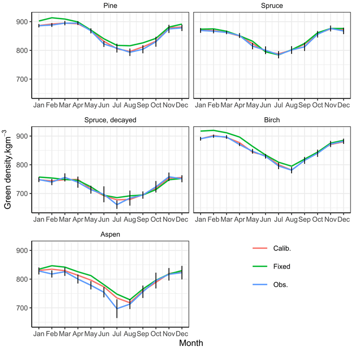
Fig. 4. Averages of observed (Obs.) and predicted (Fixed, Calib.) green density values in the test data (2019) by month. Fixed is fixed predictions. Calib. is the predictions obtained with the nationwide calibration.
For pine, spruce, and birch, nationwide calibration corrected the predictions based on the fixed part only so that they closely followed the overall seasonal variation in the measured green densities of the test data (Fig. 4). Significant improvements were also visible in the monthly averages of the decayed spruce especially in January and February and the summer months, but the calibration data were not sufficient to reveal the July downwards dip in green density. For aspen, calibration data were too small to correct the overprediction between April and July.
In most cases, nationwide calibration also ensured reliable prediction at the regional level. For example, corrections of pine green density predictions were consistent in sub-areas A to D (Table 7). However, sub-area E was an exception, where the nationwide calibration was corrected for the wrong direction. The model predictions were systematically too small from April to August, and the nationwide calibration made them worse (Fig. 5). In this case, regional calibration, i.e. calibration by applying the regional weight measurements and random week effect presented in MODEL 2, led to more reliable prediction (Fig. 5). In the other regions with a sufficiently large calibration dataset, the results of regional calibration differed little from the nationwide calibration (Table 7).
| Table 7. Differences in the annual sub-area level averages over the whole test data (year 2019) between the predicted and measured green densities (kg m–3) by pulpwood assortments; predictions both with fixed part of the model and after calibration, using the predicted week effects. | ||||
| Sub-area | N | Prediction error Mean | ||
| Fixed | Nationwide calibration | Regional calibration | ||
| A | 193 | –17.3 | –7.0 | –8.4 |
| B | 826 | –18.3 | –5.7 | –4.1 |
| C | 38 | –16.0 | –3.8 | NA* |
| D | 506 | –16.3 | –4.5 | –6.2 |
| E | 128 | 19.8 | 31.3 | 8.3 |
| N, number of observations in test data (2019); Fixed, fixed predictions of the developed models; Nationwide calibration, predictions calibrated at national level; Regional calibration, predictions calibrated at reginal level. *Could not be estimated due to low number of observations. | ||||
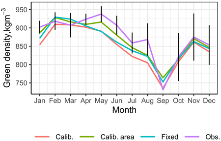
Fig. 5. Monthly averages of observed (Obs.) and predicted (Fixed, Calib. Calib_area) green density values in sub-area E (North Finland) in the test data (2019). Fixed is fixed predictions. Calib. is the predictions obtained with the nationwide calibration. Calib_area is the predictions obtained with the regional calibration.
4 Discussion
Although models or calculation methods for predicting the drying or moisture content of different timber assortments with the help of meteorological data have been employed in several studies (Liang et al. 1996; Filbakk et al. 2011; Gigler et al. 2000; Murphy et al. 2012; Routa et al. 2012; Erber et al. 2014; Raitila et al. 2015; Routa et al. 2015a, 2015b; Routa et al. 2016; Lindblad et al. 2018), the effects of storing and weather conditions on the green density of timber has rarely been studied and published. Hultnäs et al. (2012) developed a statistical model that could predict the green density of Norway spruce pulpwood by using density data from earlier years for a certain mill and meteorological data from the wood supply area of the mill. In a study that can be considered as preliminary to the present one, Lindblad and Repola (2019) presented mixed models for the green density of pine and birch pulpwood in terms of measurement time and storage period.
The present study was aimed at models that could be operationalized in determining the green density value of pulpwood arriving at mills. Linear mixed models with both fixed and random parameters were developed for the green density (kg m–3) of the different pulpwood assortments (pine, spruce, decayed spruce, birch, and aspen). The fixed effect predicted the overall expected value of green density as a function of delivery date, storage time, and meteorological conditions during storage. In addition, when only delivery date is available the complementary models based only delivery date were developed. The random effects allowed temporal calibration by utilizing the most recent sampling weight measurements. The developed models for pine and birch were based partly on the same material used in the study of Lindblad and Repola (2019), but the material was completed with the new observations (2017–2019) and the meteorological data.
Temporal correlations in the residuals of the fixed part were modeled in a coarse scale by including the autocorrelated random week effects. Regional MODELS 2 were provided to account for large-scale spatial variation in the residuals. Arguably, a more realistic description and more efficient prediction of spatial-temporal variation in green density could be achieved by models with smoothly varying spatial and temporal effects. In this study, the choice of coarse scales was motivated by the requirements imposed on the operational system: In discrete space-time, we can determine a sample size of calibration data such that the random effects can be predicted with a given precision. In practice, sample size can be controlled on a weekly basis, but it would be impractical for spatial units smaller than those of Fig. 2.
The model validation showed that the developed models provided a realistic description of the observed seasonal variation in green density, and that the model predictions were more reliable than those obtained with current practices. Even the uncalibrated (fixed) predictions led to lower relative root mean squared prediction errors (rRMSE), indicating a lower deviation of the single bundles from the measured values compared with values obtained with the currently used practices (mill-specific trimmed moving averages of sample weight measurement or fixed green density factors). The importance of temporal calibration was revealed when the rRMSE was calculated from weekly averages, and when monthly or annual averages of predictions were compared with the averages of measured green densities.
Although the developed models produced a low rRMSE compared with the current methods, that alone was not a sufficient guarantee for the predictions to be reliable throughout the year, especially when the model is applied to new data. In practice, the aim is to apply the developed models to new weight measurements in the upcoming years. The seasonal trends or the general level of green density values can then deviate systematically from that of the modeling data. In this case, the fixed effect of the models can lead to poor predictions. This was already evident in the model validation with test data (2019). For this reason, the models were specified so that it could be calibrated flexibly in a short interval with the sample weight measurements of new observations. In the model validation, the predictions were calibrated with predicted random week effects based on the sample weight measurements of the previous four weeks. This procedure proved an effective way to correct the fixed predictions to the current level. The default calibration was based on the common random effect for the whole country. Although such nationwide calibration produced reliable predictions at the country level, this was not the case for all parts of the country. The test data showed that nationwide calibration even increased the prediction error in sub-area E (Lapland), where the observed green density values in 2019 were systematically at a higher level than in the other sub-areas. In this case, regional calibration, by applying the regionally predicted random effects and only the observations within the sub-area, was needed to improve the predictions.
Our validation experiments thus revealed that the green density predictions obtained with the fixed part of the model alone cannot be expected to be sufficiently reliable for practical purposes. Nationwide, and when necessary regional, calibration must be applied to obtain the required accuracy of the predictions. This also requires that the sampling used to collect up-to-date calibration data must be controlled to ensure sufficient coverage of timber from different regions and seasons, as well as with different storage times. Our test data appeared to be clearly sufficient for the successful national calibration of the main assortments (pine, spruce, and birch), with approximately 30 samples per week on average. On the other hand, a lack of data was evident in the national calibration of aspen and the regional calibration of pine in regions A, C, and E (less than six samples per week on average). An important advantage of the linear mixed model predictions is that they come with an estimate of the prediction uncertainty which can in turn be utilized to adjust the future sampling density so that it is anticipated to yield sufficiently precise predictions.
To ensure the suitability of the models in practice, only the variables (delivery date, storage time, and meteorological conditions during storage) that were commonly available, or which could be estimated easily and reliably from the database, were used as predictors. Of the meteorological variables, wind and humidity could not be used, because they were not available for the observations measured before 2016. Green density and wood drying are also known to be affected by many other factors such as wood basic density, the amount of heartwood, the storage condition at the roadside, the amount of bark in logs, and the moisture content of the standing tree (Hakkila 1966; Hakkila 1979; Kokkola 1993; Persson et al. 2002; Routa et al. 2015b). These factors could not be accounted for in our models. However, as illustrated in this paper, such deficiencies in the fixed part of the model can be compensated by the possibility of efficiently calibrating the random part.
The seasonal trends of green density values were detected for all pulpwood assortments. The green density was highest in the timber delivered during the winter months, decreased during the spring months, and was lowest in the summer months. Similar trends were also observed in previous studies (Hautamäki et al. 2010; Hultnäs et al. 2012; Lindblad and Repola 2019). Hultnäs et al. (2012) used seasonal dummy variables to describe such a seasonal trend for spruce pulpwood by classifying the year into 24 groups. In this study, the week number (1–53) with different power transformations was used as a continuous predictor to describe the seasonal variation. The use of a continuous, rather than categorical, variable increased model precision and flexibility especially in the season (the spring months in our case) when the change in green density values was rapid. The storage time (STORAGE) had an influence on the wood drying of all pulpwood assortments. Green density showed a decreasing trend as a function of storage time even though the drying effect diminished with long storage time and in the winter months. In general, both temperature and precipitation during storage had a significant effect on green density: temperature had a positive and precipitation a negative effect on wood drying. Hultnäs et al. (2012) reported that the effect of weather conditions (temperature, precipitation, wind) was significant only for wood delivered in the spring and summer months. These results are not directly comparable with our study, because we used meteorological variables determined over the exact storage time, whereas Hultnäs et al. (2012) used weather conditions determined by two-week periods analogously with the delivery date.
In addition to appropriate specification, the reliability and applicability of the models also depends on representative study material. The data should have a high variation of independent variables, which is a prerequisite for a reliable regression model (Mehtätalo and Lappi 2020). The developed models were based on the large (N = 46 073) and encompassing material collected between 2013–2018 in mills (N = 17) located in different parts of Finland covering almost the whole country and composing a significant share of pulpwood flow in Finland. Owing to the timespan of several years and good areal coverage, there was a high variation of the independent variables, which enabled a reliable parameter estimation and widely applicable model for the current pulpwood flow in Finland.
The current fixed conversion factors, the “green density tables”, are divided into five large regions, containing several sub-regions. The regions are Southern Finland, Ostrobothnia, Kainuu, Lapland, and Northern Lapland. However, the same conversion factor can be applied for regions as large as 300 km × 400 km. The current green density factors are based on long-term average values and fixed for seasons and geographical areas. As a result, local or between-timber parcel variation in wood properties is not considered in this approach. Furthermore, fixed conversion factors are insensitive to the local or even sub-regional effects of weather conditions; the geographical or between-year variability of weather conditions can lead to a remarkable difference between fixed and observed green density.
Since the beginning of 2018, it has been possible to use weather-based moisture content estimation models in connection with the weight measurement of harvesting residues. Thus far, this is the only and first timber measurement method in Finland in which real meteorological observations have been utilized. The introduction of the method and green density estimation models presented in this study would be a significant change in pulpwood measurement and in the use of meteorological data in timber measurement in general. Utilizing gridded weather data facilitates the use of models at every location in Finland. The disadvantages of this method are that it cannot take into consideration any site-specific meteorological effects that influence green density. The further development of the method and green density models is possible by using the measurement data collected in connection with weight sampling measurement. However, a key precondition is that more quantities that can reasonably be attributed to the storage conditions and properties of the timber are available. Knowing the exact location of the timber origin would improve the match of the weather observations with the timber lots. In addition, it is possible to include new meteorological variables in the models. Knowledge of forest site types, the type of felling, and the dimensions of timber would allow the models to be developed in terms of the timber’s characteristics.
Openness of research data
The study material was obtained from the pulp mill companies and it is confidential or not available without separate permission. The used statistical code (SAS, R) are available on request from the authors.
Authors’ contribution
Project administration, data acquisition and processing, Jari Lindblad; statistical methodology (model calibration), Juha Heikkinen; model estimation, Jaakko Repola. All authors contributed to scientific writing and the revisions of the manuscript and have agreed to the published version of the manuscript.
Acknowledgments
The authors wish to acknowledge Metsäteho Ltd., Stora Enso Ltd., UPM-Kymmene Ltd. and Metsä Group for their good cooperation, contribution and financial support. The authors appreciate the anonymous reviewers for constructive comments and suggestions. The authors would also like to thank Mr. Rupert Moreton, Acolad for revising the language.
Funding
This study was financially supported by Stora Enso Ltd., UPM-Kymmene Ltd., Metsä Group and Natural Resources Institute Finland.
References
Aalto J, Pirinen P, Heikkinen J, Venäläinen A (2013) Spatial interpolation of monthly climate data for Finland: comparing the performance of kriging and generalized additive models. Theor Appl Climatol 112: 99–111. https://doi.org/10.1007/s00704-012-0716-9.
Erber G, Routa J, Kolström M, Kanzian C, Sikanen L, Stampfer K (2014) Comparing two different approaches in modelling small diameter energy wood drying in logwood piles. Croat J For Eng 1: 15–22. https://hrcak.srce.hr/120234.
Filbakk T, Hoibo O, Dibdiakova J, Nurmi J (2011) Modelling moisture content and dry matter loss during storage of logging residues for energy. Scand J Forest Res 26: 267–277. https://doi.org/10.1080/02827581.2011.553199.
Gigler J, van Loon W, Seres I, Meerdink G, Coumans W (2000) PH—Postharvest Technology: drying characteristics of willow chips and stems. J Agr Eng Res 77: 391–400. https://doi.org/10.1006/jaer.2000.0590.
Hakkila P (1966) Investigation on the basic density of Finnish pine, spruce and birch wood. Commun Inst For Fenn 61: 1–98. http://urn.fi/URN:NBN:fi-metla-201207171093.
Hakkila P (1979) Wood density surveys and dry weight tables for pine, spruce and birch stems in Finland. Commun Inst For Fenn 96. http://urn.fi/URN:ISBN:951-40-0470-1.
Hautamäki S, Kilpeläinen H, Sirkiä S, Verkasalo E (2010) Moisture development behaviour and models applicable for pulpwood and round energywood assortments in Finland. In: Asplund D, Savolainen M (eds) Forest Bioenergy 2010, From 31st August to 4th of September 2010, Tampere, Finland, Book of Proceedings. FINBIO Publications 47, pp 171–178.
Heikkilä J, Lindblad J, Hujo S, Verkasalo E (2004) Pienten kuitupuuerien mittaus puutavara-auton kuormainvaa’alla. [Measurement of small parcels of pulpwood using the weighing equipment mounted on the crane of timber truck]. Metsätieteen aikakauskirja 4/2004: 527–540. https://doi.org/10.14214/ma.5669.
Hultnäs M, Nylinder M, Ågren A (2012) Predicting the green density as a means to achieve the volume of Norway spruce. Scand J Forest Res 28: 257–265. https://doi.org/10.1080/02827581.2012.735697.
Kokkola J (1993) Drying of pulpwood in northern Finland. Silva Fenn 27: 283–293. https://doi.org/10.14214/sf.a15683.
Liang T, Khan MA, Meng Q (1996) Spatial and temporal effects in drying biomass for energy, Biomass Bioenerg 10: 353–360. https://doi.org/10.1016/0961-9534(95)00112-3.
Lindblad J, Repola J (2019) Mänty- ja koivukuitupuun tuoretiheys paino-otantamittauksessa ja tuoretiheyden mallinnus varastointiajan perusteella. [Green density of pine and birch pulpwood in the sampling-based weight measurement and modelling of green density based on storage time]. Metsätieteen aikakauskirja, article id 10101. https://doi.org/10.14214/ma.10101.
Lindblad J, Routa J, Ruotsalainen J, Kolström M, Isokangas A, Sikanen L (2018) Weather based moisture content modelling of harvesting residues in the stand. Silva Fenn 52, article id 7830. https://doi.org/10.14214/sf.7830.
McCulloc CE, Searle SR (2001) Generalized, linear and mixed models. Wiley, New York. https://doi.org/10.1002/0471722073.scard.
Mehtätalo L, Lappi J (2020) Biometry for forestry and enviromental data: with examples in R. Chapman and Hall/CRC. https://doi.org/10.1201/9780429173462.
Melkas T (2020) Wood measuring methods used in Finland 2019. Metsäteho Result Series 3-EN/2020. https://www.metsateho.fi/wood-measuring-methods-used-in-finland-2019/.
Murphy G, Kent T, Kofman PD (2012) Modeling air drying of sitka spruce (Picea sitchensis) biomass in off-forest storage yards in Ireland. For Prod J 62: 443–449. https://doi.org/10.13073/FPJ-D-12-00096.1.
Natural Resources Institute Finland (2017) Luonnonvarakeskuksen määräys puutavaran mittaukseen liittyvistä yleisistä muuntoluvuista annetun Metsäntutkimuslaitoksen määräyksen liitteen muuttamisesta. [Natural Resources Institute Finland’s regulation on amending the appendix of the regulation related to the currently used conversion factors of timber measurements issued by the Finnish Forest Research Institute]. Regulation number 1/2017, Authority regulations. https://www.finlex.fi/fi/viranomaiset/normi/410001/43823.
Parresol BR (1999) Assessing tree and stand biomass: a review with examples and critical comparisons. Forest Sci 45: 573–593. https://www.fs.usda.gov/treesearch/pubs/1180.
Persson E, Filipsson J, Elowson T (2002) Roadside storage of Norway spruce (Picea abies (L.) Karst.) pulpwood – effect on moisture content of climate conditions, felling season and exposure. Pap Tim 84: 174–178.
Raitila J, Heiskanen V-P, Routa J, Kolström M, Sikanen L (2015) Comparison of moisture prediction models for stacked fuelwood. Bioenerg Res 8: 1896–1905. https://doi.org/10.1007/s12155-015-9645-7.
Routa J, Kolström M, Ruotsalainen J, Sikanen L (2012) Forecasting moisture changes of energy wood as a part of logistic management. In: Special issue, Abstracts for international conferences organized by LSFRI Silava in cooperation with SNS and IUFRO. Mezzinatne 25: 33–35.
Routa J, Kolström M, Ruotsalainen J, Sikanen L (2015a) Precision measurement of forest harvesting residue moisture change and dry matter losses by constant weight monitoring. Int J For Eng 26: 71–83. https://doi.org/10.1080/14942119.2015.1012900.
Routa J, Kolström M, Ruotsalainen J, Sikanen L (2015b) Validation of prediction models for estimating the moisture content of small diameter stem wood. Croat J For Eng 36: 283–291. https://hrcak.srce.hr/151826.
Routa J, Kolström M, Ruotsalainen J, Sikanen L (2016) Validation of prediction models for estimating the moisture content of logging residues during storage. Biomass Bioenerg 94: 85–93. https://doi.org/10.1016/j.biombioe.2016.08.019.
Sikanen L, Marjomaa J (1992) Metsätraktorin kuormainvaa’an käyttöön perustuva puutavaran tilavuuden mittaus [Timber volume measurement with forwarder’s grapple-mounted scales]. Metsätehon katsaus 14/1992. https://metsateho.fi/wp-content/uploads/katsaus-1992_14.pdf.
Venäläinen A, Heikinheimo M (2002) Meteorological data for agricultural applications. Phys Chem Earth 27: 1045–1050. https://doi.org/10.1016/S1474-7065(02)00140-7.
Total of 27 references.
