Eva Ring  ,
Fredrik Johansson,
Claudia von Brömssen,
Isabelle Bergkvist
,
Fredrik Johansson,
Claudia von Brömssen,
Isabelle Bergkvist
A snapshot of forest buffers near streams, ditches, and lakes on forest land in Sweden – lessons learned
Ring E., Johansson F., von Brömssen C., Bergkvist I. (2022). A snapshot of forest buffers near streams, ditches, and lakes on forest land in Sweden – lessons learned. Silva Fennica vol. 56 no. 4 article id 10676. https://doi.org/10.14214/sf.10676
Highlights
- Forest buffers were inventoried on 174 harvested and site-prepared compartments bordering surface water in Sweden
- Buffers with 100% shoreline coverage were present beside all 16 lakes and 55% of the natural or modified stream reaches
- Judging streams´ character from field inspection of individual reaches alone proved difficult on forest land affected by historic drainage activities.
Abstract
Forest buffers beside surface water can mitigate negative effects of logging. To gain more information on buffer implementation in operational forestry, forest buffers were inventoried during 2018 on 174 harvested and site-prepared compartments traversed by or bordering streams, ditches and lakes in three regions across Sweden 2–4 years after clearcutting. Most of the inventoried stream and ditch reaches were ≤5 m wide. The water reaches were categorized as lakes (n = 16), natural streams (n = 50), modified streams (n = 21) or ditches (n = 87). Forest buffers with 100% shoreline coverage were present along all lake reaches and 55% and 10% of the natural or modified stream and ditch reaches, respectively. Buffers were absent beside 14% of the natural or modified stream reaches and 61% of the ditch reaches. Lake reaches had significantly wider buffers on average than ditch reaches and natural or modified stream reaches. The mean (SE) buffer widths beside lakes, natural or modified stream reaches and ditch reaches across all three regions and shoreline coverage classes were 12 (1.1), 6.6 (0.6) and 1.5 (0.5) m, respectively. The character of the local stream networks (natural or modified streams or ditches) containing each inventoried reach, were assessed using map information and the reaches´ field classifications. This illustrated the difficulty of judging a streams´ character based solely on field inspections of individual reaches on forest land where historic drainage activities have been performed. We recommend that also upstream and downstream conditions should be considered when planning environmental measures to protect surface water bodies.
Keywords
forestry;
conifer;
harvest;
lake;
riparian;
stream;
watercourse
-
Ring,
Skogforsk (The Forestry Research Institute of Sweden), Uppsala Science Park, 751 83 Uppsala, Sweden
 https://orcid.org/0000-0002-8962-9811
E-mail
eva.ring@skogforsk.se
https://orcid.org/0000-0002-8962-9811
E-mail
eva.ring@skogforsk.se
- Johansson, Skogforsk (The Forestry Research Institute of Sweden), Uppsala Science Park, 751 83 Uppsala, Sweden E-mail fredrik.johansson@skogforsk.se
-
von Brömssen,
Department of energy and technology, Division of applied statistics and mathematics, Swedish University of Agricultural Sciences, 750 07 Uppsala, Sweden
https://orcid.org/0000-0002-1452-8696
E-mail
Claudia.von.Bromssen@slu.se
- Bergkvist, Mellanskog, Uppsala Science Park, Box 127, 751 04 Uppsala, Sweden E-mail isabelle.bergkvist@mellanskog.se
Received 20 December 2021 Accepted 26 September 2022 Published 8 December 2022
Views 54787
Available at https://doi.org/10.14214/sf.10676 | Download PDF

Supplementary Files
1 Introduction
Forest buffers are strips of riparian forest that are deliberately left near surface waters to mitigate or avoid negative impacts of logging, in both the buffers themselves and the adjacent waters (Broadmeadow and Nisbet 2004; Gundersen et al. 2010; Hylander and Weibull 2012; Oldén et al. 2019b). The delineation and characteristics of forest buffers determine their functions and the level of protection they provide (Clinton 2011; Sweeney and Newbold 2014; Lidman et al. 2017; Jyväsjärvi et al. 2020). A forest buffer´s width is one of several important factors that affect not only its functions but also the forest owner´s profitability (Sonesson et al. 2021). Consequently, there have been strenuous efforts to establish sufficient widths for maintaining various environmental functions (Broadmeadow and Nisbet 2004; Clinton 2011). Fixed width buffers have commonly been used in operational forestry, but the use of variable buffer widths has also been proposed (Richardson et al. 2012; Kuglerová et al. 2014).
A previous study of policy settings in seven Nordic-Baltic countries showed that both legislation and voluntary commitments play important roles in the implementation of protection zones for forest waters (Ring et al. 2017). The degree of prescriptiveness and relative importance of voluntary or mandatory commitments varied between countries, apparently in part because of differences in land-use distributions and forest ownership structures as well as historical and political legacies. It was not possible to relate differences in policy to differences in practical implementation because of the paucity of national statistics on forest buffers. In Sweden and Finland, implementation of protection zones was found to rely heavily on voluntary commitments. Based on a recent study of small streams in Sweden, Finland and British Columbia in Canada, Kuglerová et al. (2020) concluded that the majority of the inventoried streams were insufficiently protected. An examination of historic data on forest buffers beside surface waters in Northern Sweden covering a 50-year period (1960s to 2013) showed that buffer implementation has varied over time (Hasselquist et al. 2020).
A longstanding governing principle of forest management in Sweden is “freedom with responsibility”, which means that the Swedish Forestry Act sets the minimum requirements for consideration of all forest values (Hasselquist et al. 2020). Forest owners have considerable freedom to decide how to meet the timber production and environmental goals laid out in the Swedish Forestry Act in practice (Hasselquist et al. 2020). Measures that are required or recommended to protect forest waters from negative effects of forestry are specified in the Swedish Forestry Act (Swedish Forest Agency 2022), forest certification standards (FSC-STD-SWE-03-2019 SW and PEFC SWE 002:4), strategic management objectives (Andersson et al. 2013, 2016; Andersson and Forsberg 2019) and both company and agency guidelines. In the Forestry Act, protection zones are defined as areas needed to prevent or limit harmful effects on adjacent environments when managing forest (Swedish Forest Agency 2022). According to the Act, protection zones containing trees and shrubs must be left when managing forest to the extent necessary with regard to species, water quality, cultural heritage values and landscape perceptions, use and outdoor recreation. The accompanying guidelines state that protection zones with regard to water quality and species in and around seas, lakes, watercourses and wet sites such as wetlands and mires should be designed based on the sensitivity and needs of species as well as soil and water conditions, and that this may be achieved for example by retaining vegetation to maintain shade and nutrient uptake and stabilize the ground (Swedish Forest Agency 2022).
In Sweden, forest land is drained by a dense hydrological network consisting of streams, ditches, rivers, wetlands and lakes. This network has been heavily affected by historic drainage activities including the digging of numerous ditches together with artificial straightening and deepening of stream reaches (Esseen et al. 2004; Hasselquist et al. 2018; Paul et al. 2022). The small-scale stream networks on forest land range from man-made ditches to natural streams. This variability suggests different needs of protection. However, the mosaic of different stream and ditch networks and their interrelations must also be considered when planning environmental measures to protect water bodies. The forest is divided into compartments (generally some hectares in size), that form the geographical basis for management and logging, but a catchment perspective is more useful when planning environmental measures to protect water. Delineating and creating functional forest buffers in this setting is challenging, particularly given the variation in the topography, soil types and forest characteristics of riparian forests. To clarify the environmental considerations and legal requirements (among others) of forestry in Sweden, the SFA initiated a dialogue process involving representatives of the SFA, other relevant authorities, operational forestry, non-governmental organizations and academia (inter alia Andersson et al. 2013). Strategic management objectives for environmental consideration have been defined (Andersson et al. 2013, 2016; Andersson and Forsberg 2019), for example regarding functional forest buffers along lakes and streams (Andersson et al. 2013). The strategic management objectives for forest buffers along lakes and streams in Sweden apply primarily to lakes and perennial streams, but also to ditches that are parts of streams, i.e., reaches that have been straightened, cleaned or deepened, excluding man-made ditches (Andersson et al. 2013). However, their application to temporary streams is also regarded as advantageous. An English translation of most of the section on forest buffers in the report by Andersson et al. (2013) has been presented by Ring et al. (2018). The strategic management objectives have been widely implemented in educational and planning material in Sweden, despite being merely recommendations (Mancheva 2021). Moreover, two forest certification standards refer to the strategic management objectives: the FSC National Forest Stewardship Standard of Sweden (FSC-STD-SWE-03-2019 SW) and the PEFC Sweden Forest standard (PEFC SWE 002:4).
There is a paucity of national statistics on forest buffers beside surface water in Sweden, but useful data on forest buffers along streams were presented by Kuglerová et al. (2020), Hasselquist et al. (2020), and Chellaiah and Kuglerová (2021). Given the importance of forest buffers for environmental protection in forestry, more information on their implementation is needed, especially since Kuglerová et al. (2020) concluded that the majority of surveyed forest buffers provided insufficient protection. Furthermore, although three previous studies have examined forest buffer implementation, all of them focused on forest buffers beside streams. Conversely, in the study presented here we inventoried forest buffers beside several different types of surface water bodies bordering regeneration cutting sites across Sweden. The presented data were collected as part of a project on mechanical site preparation near surface water whose results are reported elsewhere (Ring et al. 2020).
The aim of this study is to expand knowledge of forest buffer implementation in Sweden by providing a snapshot of the characteristics of forest buffers created during regeneration cutting conducted next to different types of commonly occurring surface water bodies. To our knowledge, forest buffers beside lakes and ditches in Sweden have not previously been studied. The results are categorized in terms of the character of the inventoried reaches bordering regeneration cutting sites, which was assessed during the field inventory; each reach was classified as a natural or modified stream, a ditch, a lake or ‘other’. However, given the historic drainage activities that have affected numerous forest surface water bodies in Sweden, they are also analysed in relation to the broader character of the streams or ditches/ditch networks to which the inventoried reaches belong, which was determined by combining data from maps with the field classifications. We hypothesize that the mean width of forest buffers is highest along water reaches seen as ’natural’, i.e., lake and natural stream reaches. Descriptive data on forest buffer shoreline coverage and canopy structure are presented and various aspects of buffer implementation are discussed, including spatial and temporal scales and issues related to the quality of the measures that are taken.
2 Materials and methods
Clear-felled compartments hosting a stream, ditch or lake were inventoried between 27 June and 22 October 2018, by five people following attendance at a calibration exercise in the field (Fig. 1). The inventory focused on 30 m wide zones bordering water. The presented data were collected as part of a project on site preparation reported by Ring et al. (2020). The aim was to survey about 300 compartments within three regions located in Sweden. The South region comprised four counties (Skåne, Halland, Kronoberg and Blekinge), the Central region comprised three counties (Uppsala, Västmanland and Örebro) and the North region comprised three counties (Jämtland, Västernorrland and Västerbotten) (Fig. 1). For inclusion in the study, compartments had to be in one of the mentioned counties, clearcut during the 2014–2015 or 2015–2016 felling periods (as identified from satellite images by the SFA, downloaded from http://geodpags.skogsstyrelsen.se/geodataport/feeds/UtfordAvverk.xml), include a water body with a shore longer than 30 m, and subjected to site preparation. Thus, the time between clear-cutting and inventory ranged between 2 and 4 years.
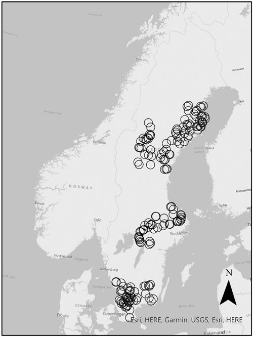
Fig. 1. Inventoried sites included in the analysis (○) in the South (n = 48), Central (n = 45) and North (n = 81) regions in Sweden. © Lantmäteriet.
2.1 Site selection
The selection of compartments began by identifying all compartments in Sweden that were clear-felled during the 2014–2015 and 2015–2016 felling periods (>100 000 sites in total) from digital maps provided by the SFA (http://skogsdataportalen.skogsstyrelsen.se/Skogsdataportalen/). Compartments hosting one or more surface water bodies were identified (24 122 sites), of which 11 156 were located within the selected regions. Surface waters located within or bordering these compartments were delineated using the vector layers of hydrography from the topographic map and delineations of water bodies and forest obtained from the Swedish Mapping, Cadastral and Land Registration Authority (https://www.lantmateriet.se/). In total, 13 328 surface waters were subsequently identified, of which 10 856 had a shore length exceeding 30 m. Along these water bodies, 2079 start positions for inventory were randomly selected using Create Random Points in ArcGIS Pro. From the list of start positions generated for each region, every 7th, 5th and 8th position (in total 72, 88 and 150 positions) were selected for waters in the South, Central and North regions, respectively. The number of start positions assigned to each region corresponded to the ratio of the summed clear-felled area in each region to the total clear-felled area in all three regions during 2014–2015 and 2015–2016 (same for both felling periods). The ratios were 22%, 29% and 48% for the South, Central and North regions, respectively. The remaining start positions were used to replace compartments that we found did not meet all the selection criteria upon arrival. Replacement compartments were selected close to those being replaced to minimize additional travelling time. The final proportions of inventoried compartments per region included in the analyses were 28%, 26% and 47% for the South, Central and North regions, respectively.
2.2 Inventory
First, the surveyor verified that the site bordered or was traversed by a stream, ditch or lake, and had undergone site-preparation. In cases where the compartment was traversed by a stream or ditch, the side of the stream or ditch hosting the largest part of the compartment was selected (Figs. 2–3). The part of the compartment shoreline to be surveyed was selected based on the distance between the start position and the compartment border in either direction (or the end of the shoreline if it ends before reaching the compartment border) (Table 1). The longest distance, henceforth referred to as the inventoried reach, was selected for inventory (Figs. 2–3). The character of the inventoried water reach, channel width and the shoreline coverage and canopy structure of the forest buffer were assessed by eye. From the start position, temporary plots (10 m wide and 30 m long, with their length being perpendicular to the shoreline) were evenly distributed along the length of each inventoried reach (Fig. 2). The number of plots depended on the length of the shoreline to be surveyed; the initial plan required 2 plots for shorelines of 30–99 m, 3 for shorelines of 100–199 m, 4 for shorelines of 200–399 m and 5 for shorelines of 400–599 m. In practice, two to three plots were inventoried at 94% of the 80 sites in the 30–99 m class (one plot was surveyed in each of the remaining five sites), three to four plots were inventoried at 94% of the 64 sites in the 100–199 m class, three to five plots were inventoried at all 26 sites within the 200–399 m class and four plots were inventoried at all four sites in the 400–599 m class. The inventory protocol is described in Table 1. The reasons why some forest buffers had incomplete shoreline coverage were not assessed. Possible reasons include selective logging or windfelling (cf. Kuglerová et al. 2020), and the presence of open wet patches containing peat. All distances other than the lengths of the inventoried shorelines were stepped out, assessed by eye or occasionally measured using measuring tape (Table 1).
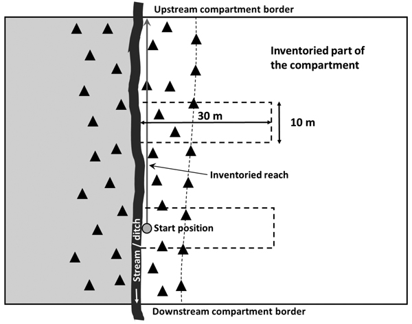
Fig. 2. Schematic illustration of the survey set-up for a compartment traversed by a stream (or ditch) with a forest buffer (the zone between the stream and thin dashed line). The side of the stream hosting the largest part of the harvested compartment was selected (white area). The grey circle shows the start position of the inventory and the attached arrow shows the inventoried reach, i.e. the longest distance from the start position to the upstream or downstream compartment border. In this example, the longest distance was to the upstream border and the distance to be inventoried was 30–99 m, requiring an inventory of two plots (indicated by dashed rectangles).
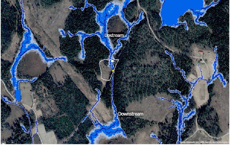
Fig. 3. Aerial photo of a compartment (dotted white line) traversed by a stream, including the up- and downstream reaches which were used for assessing the stream type. In this case, the up- and downstream reaches were classified as ‘natural’ from the map and the inventoried reach (i.e., the reach between the white and yellow circles) was categorized as ‘modified’ during the field inventory, giving the stream type ‘modified stream’. The photo is overlaid by the depth-to-water map obtained from Swedish Forest Agency (https://www.skogsstyrelsen.se/). © Lantmäteriet.
| Table 1. Inventory protocol for the forest buffer and site characteristics presented in this study including the inventoried variables, their available classes or measure and comments on the methods or classes used (see also Ring et al. 2020). | ||
| Variable | Available classes or measure | Comments |
| Character of water reach bordering the compartment | Natural stream | Assessed for the water reach traversing or bordering the compartment. A natural stream is one showing no evidence of human interference. |
| Modified stream | Modified stream: signs of human activity, for example straightened or deepened stream channel. | |
| Ditch | ||
| Lake | ||
| Wide river | ||
| Other | ||
| Inventoried shore length | Meters | Measured using a tablet computer from the start position to the border of the compartment, or end of the reach if it ends before the compartment border (determined by eye from the start position), using ’Collector for ArcGIS’ with Esri´s basemap for Sweden, based on Lantmäteriet´s open data (orthophoto), as background. |
| Channel width | Meters without decimal fractions | The channel width at the start position estimated by eye. Stream: width of stream bed with exposed mineral soil or where the vegetation shows signs of high water levels. Ditch: width at the soil surface. |
| Shoreline coverage of the forest buffer | 100% | Percentage class of the shoreline forest buffer coverage, i.e., coherent area with trees (with breast-height diameter >7 cm) spaced <10 m apart, along the entire inventoried reach. |
| 75–100% | ||
| 50–75% | ||
| <50% | ||
| No buffer | ||
| Width of forest buffer | Meters without decimal fractions | The width from the most distant tree trunk to the shoreline within the plot stepped out or assessed by eye. |
| Canopy structure of the forest buffer | Multi-layered | Canopy structure of the buffer along the entire inventoried reach. |
| Single-layered | ||
| Single trees | ||
| Shrubs | ||
| Wetland forest | ||
| Soil moisture class | 1–4 | Dry (1), mesic (2), moist (3) or wet (4). The soil moisture class determined for the first 10 m from the shoreline of the plots. |
| Surface structure class | 1–5 | Even ground (class 1) to technically impossible to harvest (class 5), determined for the plots. |
| Trafficability class | 1–5 | Very good (class 1), allowing forestry work year-round to very bad (class 5) restricting forestry work to periods with frozen ground, according to Berg (2006), determined for the plots. |
2.3 Characterization of water reaches and stream types
Each inventoried reach was characterized as a lake, natural stream, modified stream, ditch or ‘other’ during the field inventory by judging the character of the reach visible from the compartment (Table 1). The character assigned to an inventoried reach in this way is henceforth referred to as its ‘reach class’. The character of the local stream network to which each inventoried reach belongs (henceforth referred to as the ‘stream type’) was assessed after completing the inventory. Reaches bordering lakes were simply characterized as lakes. The stream type was defined by considering the reach upstream of the inventoried reach, the inventoried reach, and the downstream reach (Fig. 3). The upstream reach comprised all or most of the stream network upstream to the source, as judged from depth-to-water maps (Murphy et al. 2008). In some cases, the upstream reach contained several channels. The downstream reach started at the downstream end of the inventoried reach and ended where the character of the watercourse clearly changed, for example because of stream confluence (see downstream section in Fig. 3) or at the outlet to a lake.
The character of the upstream and downstream reaches was individually determined by visual inspection of the most recent digital orthophotos available, overlaid by the vector layer of hydrography from the topographic map, and depth-to-water maps. The orthophotos and the vector layer of hydrography were obtained from the Swedish Mapping, Cadastral and Land Registration Authority (https://www.lantmateriet.se/) and the depth-to-water maps, with 2 m × 2 m resolution, downloaded from the SFA (https://www.skogsstyrelsen.se/).
First, the direction of water flow at the start position was determined. Then the upstream and downstream reaches were classified as natural streams if they had a meandering channel sometimes starting from, and/or running through, peatland areas without ditches, and a location complying with the depth-to-water map. They were classified as modified streams if there were signs of excavation work and at least one straight reach; and ditches if the channels were largely straight and did not always comply with the depth-to-water map, suggesting that they were man-made.
The stream type was determined from the field classification of the inventoried reach and the assessments of the upstream and downstream reaches. However, if the inventoried reach was the source of the stream, only the downstream reach was considered. A stream was classified as a natural stream if all its reaches were classified as natural streams, as a ditch if all its reaches were classified as ditches, and as a modified stream if it included both ditch and natural stream stretches (Figs. 3–4). Most of the draining channels of the ditch streams were ditches, while the channels of modified streams generally had characteristics of natural streams. Forest buffer characteristics were mainly analyzed in relation to the reach class.
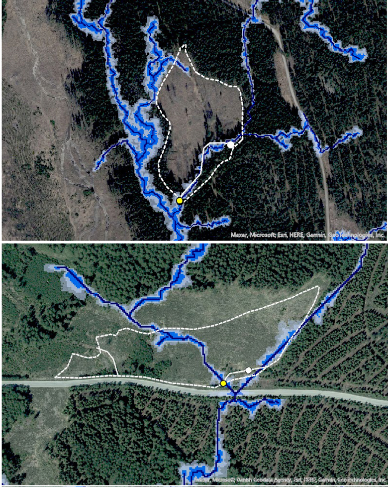
Fig. 4. Aerial photos of two inventoried sites, representing the stream types ‘natural stream’ (top) and ‘ditch’ (bottom), overlaid by the depth-to-water map obtained from the Swedish Forest Agency (https://www.skogsstyrelsen.se/). The dotted white lines indicate compartment boundaries and the solid white lines the randomly selected water reaches (obtained from the vector layer of hydrography, https://www.lantmateriet.se). White circles indicate start positions and yellow circles the end of the inventoried reaches. © Lantmäteriet.
Four reaches were categorized as ’other‘ during the inventory. One was described as a ’pond‘, and subsequently classified as lake (surrounded by a ditch) following examination of the maps. The other three reaches were wet areas at the start of a stream. Since these reaches were dominated by subsurface water flow, they were excluded from the analyses.
2.4 Data analysis
The collected data were checked and 14 records with incomplete or invalid data were removed, including the records of three compartments where the survey had been performed beyond the 30 m long plots and four duplicate records. Since the number of plots per compartment varied, arithmetic means for each compartment (henceforth referred to as compartment means) were calculated for variables determined from field observations in the plots (i.e., buffer width, soil moisture class, surface structure class, and trafficability class) and combined with field data represented by one observation per compartment (i.e., forest buffer shoreline coverage, inventoried shore length, forest buffer canopy structure and channel width). Some compartment information (for example, on size of harvested area) was also obtained from the SFA. The variables forest buffer width, inventoried shore length, channel width, size of harvested area and number of plots per compartment were fitted with linear models using reach class, region, and their interaction as fixed factors. Similar models were also generated using stream type, region and their interaction as fixed factors. Lake reaches were included in both types of models. In addition, these variables (except size of harvested area with an indicated interaction between reach class and region) were fitted with a linear model including reach class (or stream type) and region, since no significant interaction between reach class (or stream type) and region was detected. The models including three factors (reach class or stream type, region and their interaction) are henceforth referred to as Model 1 and the models including two factors (reach class or stream type and region) as Model 2. For the variables forest buffer width and number of plots per compartment, the analyses using Models 1 and 2 were performed on compartment means. Since the residuals exhibited a skewed distribution for all variables, the models were fitted using a generalized linear model with a Gaussian distribution and a logarithmic link function, which is a better option than logarithmic transformation when the observed values include zeros. The models were fitted using the GENMOD procedure in the SAS/STAT 15.2 software, Version 9.4 (TS1M7) of the SAS System for Windows. Differences between least squares means, adjusted for multiple comparisons according to the Tukey–Kramer method, were used to evaluate the significance of effects, applying a significance threshold of p < 0.05. Standard errors (SE) were calculated using the GENMOD procedure and re-transformed from logarithmic values by the delta method.
In a few cases, conflicting data were identified. More specifically, three compartments had less than 50% shoreline coverage and 0m buffer width. Thus, when determining the proportion of compartments lacking a forest buffer, the calculation was based on the number of compartments assigned to the shoreline coverage class ’No buffer‘ (rather than using a buffer width of 0m). The data included some missing observations, presented in the following text and tables as ’nna’ or ‘na’ (i.e., number or proportion with missing observations). On the compartment level (n = 174), the number of missing observations were 1, 2, 7 and 4 for forest buffer width, shoreline coverage of the buffer, buffer canopy structure and channel width, respectively. Note, that information on buffer canopy structure was registered for 26 out of 63 sites lacking a forest buffer. In these cases, the buffer canopy structure was characterized as shrubs (13 sites), single trees (12 sites) or shrubs and single trees (1 site). On the plot level (n = 496), ten plots lacked data on forest buffer width and 1–11 plots lacked data on soil moisture class, surface structure class and trafficability class.
3 Results
3.1 Surveyed compartments
As shown in Table 2, 332 compartments were visited, of which 174 were surveyed and included in the analysis. Other compartments were not surveyed for reasons presented in the table. Almost half of the total surveyed shore length (46%) was in the North region, with 24% and 30% in the South and Central regions, respectively (for more information, see Supplementary file S1). The channel width at the start positions was ≤7 m in all cases (nna = 4), except for one reach beside an approximately 80 m wide river in the North region (Table 2, Suppl. file S1). Most (70%) stream and ditch reaches were 1–2 m wide (at the start position) (na = 2.5%). According to Model 1, neither the channel width nor the inventoried shore length were significantly affected by reach class (or stream type), region or their interaction (p ≥ 0.07) (Table 3). The size of the harvested area differed significantly between regions in the stream type Model 1, but not in the reach type Model 1. There was an interaction between reach class and region indicating larger harvested compartments near lake reaches than ditch and possibly natural stream (p = 0.065) reaches in the North region. The number of inventoried plots per compartment differed between regions in both the reach class and stream type Model 1 (Table 3). The mean number of plots was higher (p < 0.01) for the South region than for the Central and North regions both in the reach class and stream type Models 2 (cf. Table 2).
| Table 2. Information regarding the compartment selection, number of inventoried plots, compartment soil characteristics, surveyed shore lengths, channel widths and number of inventoried lake, stream and ditch reaches (or stream types). The data were collected for three regions (South, Central and North) in Sweden and are presented per region and in total. ‘Mean’ denotes the arithmetic mean and ‘SE’ the sample standard error. | ||||
| South region | Central region | North region | Total | |
| No. of visited compartments | 104 | 93 | 135 | 332 |
| No. of surveyed compartments | 48 | 45 | 81a | 174 |
| No. of unsurveyed compartments | 56 | 48 | 54 | 158 |
| Reason for not surveying: | ||||
| – not site-prepared | 46 | 22 | 31 | 99 |
| – could not be reached | 7 | 16 | 16 | 39 |
| – lacked a water body | 1 | 0 | 2 | 3 |
| – other | 1 | 9 | 4 | 14 |
| – no reason stated | 1 | 1 | 1 | 3 |
| All data presented below refer to compartments included in the analysis | ||||
| No. of inventoried plots per compartment: | ||||
| Mean | 3.3 | 2.8 | 2.6 | 2.9 |
| Min–max | 2–5 | 2–4 | 1–4 | 1–5 |
| No. of inventoried plots in total | 157 | 125 | 214 | 496 |
| Size of surveyed harvested compartments: | ||||
| Mean (ha) | 3.5 | 6.7 | 9.1 | 6.9 |
| Min–max (ha) | 0.2–11.9 | 0.7–40.2 | 0.6–45.2 | 0.2–45.2 |
| Trafficability classb– mean (SE) | 2.4 (0.1) | 2.6 (0.1) | 2.5 (0.1) | 2.5 (0.07) |
| Surface structure classb– mean (SE) | 1.6 (0.08) | 1.6 (0.07) | 1.4 (0.07) | 1.5 (0.04) |
| Soil moisture classb,c– mean (SE) | 2.4 (0.06) | 2.4 (0.09) | 2.9 (0.06) | 2.6 (0.04) |
| Surveyed shore length: | ||||
| Mean (m) | 105 | 143 | 122 | 123 |
| Min–max (m) | 23–500 | 50–470 | 20–480 | 20–500 |
| Total (km) | 5.0 | 6.4 | 9.9 | 21.3 |
| Channel width (at the start position) for streams and ditches: | ||||
| Mean (m) | 2.1 | 1.8 | 3.2 (2.1)d | 2.5 (2.0)d |
| Min–max (m) | 1–7 | 1–4 | 0–80 (0–6)d | 0–80 (0–7)d |
| Type of water, no. per category (reach class / stream type): | ||||
| Natural stream | 6 / 3 | 5 / 3 | 39 / 23 | 50 / 29 |
| Modified stream | 9 / 25 | 9 / 26 | 3 / 43 | 21 / 94 |
| Ditch | 27 / 14 | 28 / 13 | 32 / 8 | 87 / 35 |
| Lake | 6 | 3 | 7 | 16 |
| a Including two compartments compartments which had not been site-prepared but had all relevant data. b See Table 1 for definitions of classes. c Determined for the first 10 m from the shoreline of the plots. d Value when the 80-m wide river was excluded. | ||||
| Table 3. Results from the statistical analyses according to Models 1 and 2 using the GENMOD procedure in SAS software. The denominator degrees of freedom were 3 for reach class and stream type, 2 for region and 6 for the interaction between reach class (or stream type) and region, except for channel width with 2 degrees of freedom for reach class (or stream type) and 4 degrees of freedom for the interaction with region. Effects were regarded statistically significant if p < 0.05. | ||||||
| Dependent variable | Factor | Chi-square statistics | p-value | Factor | Chi-square statistics | p-value |
| Model 1 | ||||||
| Forest buffer width | Reach class | 37.5 | <0.01 | Stream type | 30.1 | <0.01 |
| Region | 0.10 | 0.95 | Region | 0.1 | 0.93 | |
| Reach class × Region | 2.0 | 0.92 | Stream type × Region | 1.6 | 0.95 | |
| Inventoried shore length | Reach class | 7.2 | 0.066 | Stream type | 2.1 | 0.56 |
| Region | 2.6 | 0.27 | Region | 3.3 | 0.19 | |
| Reach class × Region | 2.8 | 0.83 | 2.6 | 0.86 | ||
| Channel width | Reach class | 0.3 | 0.84 | Stream type | 0.5 | 0.79 |
| Region | 0.03 | 0.98 | Region | 0.9 | 0.64 | |
| Reach class × Region | 0.1 | 1.0 | Stream type × Region | 0.2 | 0.99 | |
| Size of harvested area | Reach class | 0.5 | 0.93 | Stream type | 0.3 | 0.96 |
| Region | 0.8 | 0.67 | Region | 6.6 | 0.036 | |
| Reach class × Region | 13.4 | 0.037 | Stream type × Region | 11.3 | 0.078 | |
| No. of plots per compartment | Reach class | 5.3 | 0.15 | Stream type | 2.3 | 0.52 |
| Region | 13.7 | <0.01 | Region | 7.9 | 0.020 | |
| Reach class × Region | 4.2 | 0.65 | Stream type × Region | 3.2 | 0.79 | |
| Model 2 | ||||||
| Forest buffer width | Reach class | 78.9 | <0.01 | Stream type | 60.4 | <0.01 |
| Region | 0.4 | 0.83 | Region | 0.05 | 0.98 | |
| Inventoried shore length | Reach class | 6.0 | 0.11 | Stream type | 1.6 | 0.65 |
| Region | 3.8 | 0.15 | Region | 4.0 | 0.14 | |
| Channel width | Reach class | 1.2 | 0.55 | Stream type | 3.3 | 0.19 |
| Region | 0.4 | 0.83 | Region | 0.8 | 0.66 | |
| No. of plots per compartment | Reach class | 5.7 | 0.13 | Stream type | 1.6 | 0.65 |
| Region | 19.3 | <0.01 | Region | 16.4 | <0.01 | |
During the field inventory, 50, 21 and 87 reaches were categorized as natural streams, modified streams, and ditches, respectively (Table 2). When assessing the stream type to which the individual reaches belonged, there were 29 natural streams, 94 modified streams and 35 ditches or ditch networks. The North region hosted a higher proportion of reaches classified as natural streams, and a lower proportion of modified streams, than the other two regions (Table 2). ‘Ditch’ was the most common type of reach (n = 87), but only 35 ditch reaches were judged to exist within streams of the ditch stream type; the other 52 were assigned to the ’modified stream’ stream type.
3.2 Forest buffer characteristics
Reach class and stream type had significant effects on forest buffer width (p < 0.01), but no effect of region or the interaction between region and reach class (or region and stream type) was detected using Model 1 (p ≥ 0.92) (Table 3, Fig. 5). According to both the reach class and stream type Models 2, forest buffers were significantly wider beside lakes than natural and modified stream or ditch reaches. The mean width of buffers beside lake, natural stream, modified stream and ditch reaches across all regions was 12, 7.9, 4.6 and 1.5 m, respectively (Table 4). The reach class and stream type Models 2 yielded different results for streams and ditches. According to the reach class Model 2, the mean buffer width for natural stream reaches was not significantly different (p = 0.11) from that of modified stream reaches but was greater than that for ditch reaches (p < 0.01). Conversely, according to the stream type Model 2, the mean buffer width for the natural stream type was greater than for the modified stream type (p < 0.01) but not significantly different to that for the ditch stream type (p = 0.10). For modified streams and ditches, a significant difference in the mean buffer width was detected according to the reach class Model 2 (p = 0.02) but not the stream type Model 2 (p = 0.41). Since many ditch reaches and ditch stream types lacked a buffer (i.e., their buffer width was 0m) (Table 4), the high proportion of zeros may have impaired model performance.
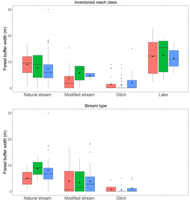
Fig. 5. Boxplots of forest buffer width for the South (red), Central (green) and North (blue) regions in Sweden by reach class (above) and stream type (below), based on compartment means. Boxes show the 25% and 75% percentiles, with a thick horizontal line and diamond indicating the median and arithmetic mean, respectively. The vertical bars show the minimum and maximum values unless observations deviate by more than 1.5 times the interquartile range (i.e., the difference between the 75th and 25th percentiles). In such cases, these observations are indicated with points.
| Table 4. Mean widths of forest buffers for the indicated classes of inventoried reaches in the South, Central, and North regions of Sweden and for all regions together, calculated by the least squares mean method using Models 1 and 2. The last two columns show the proportion lacking a forest buffer and the proportion containing buffer covering 100% of the surveyed reach for all three regions together. Mean = least squares mean calculated using the GENMOD procedure in SAS software, SE = standard error calculated using the GENMOD procedure and re-transformed from logarithmic values using the delta method, n = sample size | ||||||
| Inventoried reach class | Forest buffer width (m) | Proportion lacking a buffer (%) | Proportion with 100% shoreline coverage (%) | |||
| Mean (SE) | ||||||
| n | ||||||
| Southa | Centrala | Northa | All regionsb | All regions | All regions | |
| Natural stream | 9.0 (1.8) | 7.8 (2.0) | 7.3 (0.7) | 7.9 (0.8) | 12c | 64c |
| 6 | 5 | 39 | 50 | |||
| Modified stream | 3.7 (1.5) | 5.7 (1.5) | 4.7 (2.6) | 4.6 (1.0) | 19 | 33 |
| 9 | 9 | 3 | 21 | |||
| Natural and modified streams | 5.8 (1.2) | 6.4 (1.2) | 7.2 (0.7) | 6.6 (0.6) | 14c | 55c |
| 15 | 14 | 42 | 71 | |||
| Ditch | 1.4 (0.9) | 1.1 (0.8) | 2.0 (0.8) | 1.5 (0.5) | 61c | 10c |
| 27 | 28 | 32d | 87d | |||
| Lake | 12.1 (1.8) | 12.4 (2.6) | 11.4 (1.7) | 12.0 (1.1) | 0 | 100 |
| 6 | 3 | 7 | 16 | |||
| a Least squares means and SE were calculated using Model 1. b Least squares means and SE were calculated using Model 2. c nna = 1 (for shoreline coverage) corresponding to 1–2% of the sample. d nna = 1. | ||||||
The proportion of inventoried reaches without a forest buffer across all regions declined in the following order: ditch reaches (61%) – modified stream reaches (19%) – natural stream reaches (12%) – lake reaches (0%) (Table 4). The proportion of reaches with 100% shoreline coverage increased in the same order. The same patterns were seen for stream types; among inventoried reaches whose stream types were ditch, modified stream, and natural stream, the proportions lacking a buffer were 71%, 38% (na = 2.1%) and 7%, respectively. When the natural and modified stream types were combined into a single group, 31% lacked a buffer and 37% had a buffer with 100% shoreline coverage (na = 1.6%).
The dataset presented here was unsuitable for detecting relations between forest buffer width and channel width, since the channel width was assessed in meters without decimal fractions (Table 1) and displayed a skewed distribution with 70% of the stream and ditch channels being 1–2 m wide (na = 2.5%). The relations between buffer and channel widths are presented graphically in Suppl. file S1.
Forest buffers covered 100% of the shoreline of all 16 lake reaches. Ten of these buffers were multi-layered and three were single-layered (nna = 3). Just over 50% of the natural and modified stream reaches (treating natural and modified streams as a single class) had 100% shoreline coverage (Table 4). About 60% of the forest buffers covering 100% of the shoreline beside natural and modified stream reaches were multi-layered, while 18% were single-layered (nna = 2.6%). A plurality of buffers beside ditch reaches (35 out of 87, na = 3, including all buffer coverage classes) were described as consisting of single trees and/or shrubs. Ditch reaches accounted for the greatest proportion of compartment reaches with no forest buffer or with a buffer having <50% or 50–75% coverage (Fig. 6). Among inventoried reaches with high shoreline coverage (≥75%), natural stream reaches dominated. More information on the buffer width is presented in the Suppl. file S1.
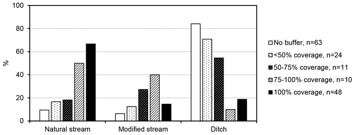
Fig. 6. Proportions of inventoried reaches in the forest buffer shoreline coverage classes no buffer, <50% coverage, 50–75% coverage, 75–100% coverage and 100% coverage (nna = 2). ‘n’ indicates the number of observations in each class.
4 Discussion
In Sweden, the hydrological network draining forest land has been heavily affected by historic drainage activities (Esseen et al. 2004; Hasselquist et al. 2018; Paul et al. 2022). Isolated ditches and straightened and deepened stream reaches that have not been maintained may today be viewed as a part of the natural hydrological network. Ditches that were dug to enable forest production in areas which would otherwise have been too wet must sometimes be maintained to provide sufficient drainage (Sikström and Hökkä 2016). This dramatically changes the conditions in the ditches, and raises needs to rigorously consider protective measures that may be required to mitigate adverse changes such as increases in sediment transport (Nieminen et al. 2018). In the longer term, maintaining shade over ditches may reduce the rate of revegetation in the ditches, and thereby reduce the need for ditch cleaning with subsequent sediment transport (Andersson and Forsberg 2019). Hence, to keep ditches shaded, the practical guidelines provided with the strategic objectives for ditch cleaning recommend only pre-harvesting the trees and shrubs needed to enable access by the ditch-cleaning machinery (Andersson and Forsberg 2019). In contrast, the strategic management objectives for forest buffers along lakes and streams were defined with the aim of maintaining the ecological functions of Sweden´s lakes, streams and riparian forests (Andersson et al. 2013). When planning environmental measures to protect surface waters in Swedish forests, it is important to understand the character of the hydrological network so that the need for protection can be accurately assessed. Deeper knowledge of the ecological role of ditches in forest landscapes could thus support the development of more effective protective measures (cf. Hasselquist et al. 2018; Paul et al. 2022).
We hypothesized that the mean width of forest buffers is highest along water reaches seen as ’natural’, i.e., lake and natural stream reaches. Lake reaches had significantly wider buffers than natural and modified stream and ditch reaches, and their buffers covered 100% of the shoreline without exception. This suggests that lakes were better protected than natural and modified streams and ditches, but it is important to recall that only 16 lake reaches were included in the study. Furthermore, natural stream reaches tended to have wider buffers than modified stream (p = 0.11) and ditch reaches (p < 0.01) (Table 4, Fig. 5). Additionally, the proportion of natural stream reaches without a forest buffer was lower than that for modified stream reaches, whereas the proportion of natural stream reaches with 100% shoreline coverage was higher than that for modified stream reaches (Table 4), suggesting that natural stream reaches have a somewhat higher level of protection than modified stream reaches, and a substantially higher level of protection than ditch reaches.
In addition to transporting water (and thus also transporting nutrients, sediments, litter, seeds, and so on), the hydrological network provides transport routes and habitats for organisms (Tolkkinen et al. 2020). This provides a simple but useful starting point for planning environmental management measures for water bodies. Forestry operations are performed on relatively small units (compartments) distributed across the landscape (cf. Table 2) and the shore lengths surveyed in this work were comparatively short – between 20 and 500 m (Table 2). Therefore, to obtain a broader hydrographic perspective, we also classified the nature of the wider stream networks to which each surveyed reach belonged (Figs. 3–4). This classification process was largely based on publicly available maps and could thus be incorporated into the practical planning of forestry operations. Although this subjective procedure requires further development (for example to account for differences in the relative lengths of the different reaches considered when evaluating the stream type), the results obtained indicate that the properties of individual reaches may not be representative of the stream in which they belong. Therefore, basing water management practices on the conditions within a focal compartment could lead to the selection of sub-optimal environmental measures. The results also suggested that the implementation of forest buffers had been influenced by the character of the inventoried reaches without accounting for the character of the up- and down-stream reaches. For example, of 63 reaches lacking a forest buffer, 53 were categorized as ditches in the field but stream type classification suggested that 28 of these reaches were actually components of modified streams. As such, they should perhaps have been protected by forest buffers. These results indicate that up- and downstream conditions should be taken into consideration when determining the need for a forest buffer. However, it is not currently clear which factors or indicators determine how much of the up- and downstream regions should be considered. In this work, the source of the stream (or ditch) and its first clear change in character downstream were used to define the limits of the upstream and downstream reaches, respectively, and the degree of anthropogenic physical impact was used as an indicator (Figs. 3–4).
The impact of forest buffers on nearby streams is related to their width, shoreline coverage, tree-species composition, age structure, type of canopy layer and stream size (Broadmeadow and Nisbet 2004; Jyväsjärvi et al. 2020; Chellaiah and Kuglerová 2021). Buffers about 10 m wide have often been found to be sufficient for preserving streams´ physical and chemical characteristics (Broadmeadow and Nisbet 2004; Clinton 2011). However, wider buffers, of at least ca. 30 m are often needed to maintain ecological values in streams and riparian zones (Kiffney et al. 2003; Sweeney and Newbold 2014; Oldén et al. 2019a,b). Of the buffers beside the natural and modified stream reaches examined in this study, 79% had mean buffer widths (compartment means) below 10 m when all shoreline coverage classes were included (cf. Fig. 5). The mean width for buffers beside natural and modified stream reaches (as a combined group) across all three regions (6.6 SE 0.6 m) was higher than the mean width (4 ± 0.4 m for 111 stream reaches in Sweden) obtained in another inventory study (Kuglerová et al. 2020). However, the mean width for the natural and modified stream types (as a combined group) was similar to that reported previously (4.6 SE 0.5 m). As shown in Table 4, the proportions of natural and modified streams found to lack a buffer in this study (14% for reaches) were higher than the proportion (5% of streams) reported by Kuglerová et al. (2020). Further, Kuglerová et al. (2020) found that forest buffers were wider on average in North Sweden (5.3 ± 0.6 m) than in the southern part (2.3 ± 0.3 m), although this was not statistically confirmed. In the present study, the mean widths for buffers beside natural and modified streams (combined) were 7.2 (0.7) and 5.8 (1.2) m in the North and South region, respectively (Table 4). We are unable to explain why greater mean buffer widths were found in the present study than in the study by Kuglerová et al. (2020). However, it is important to also take account of other forest buffer characteristics in addition to width (Chellaiah and Kuglerová 2021).
Results of this study provide a snapshot of some characteristics of forest buffers in Sweden. Forest buffer width, proportion of sites lacking a buffer, shoreline coverage and canopy structure are useful measures for evaluating buffer status in an area, region or country. However, the policy setting in Sweden leaves substantial room for individual interpretation and forest buffer implementation may be seen as a long-term process (Andersson et al. 2013; Hasselquist et al. 2020). Forest buffers began to be implemented in Swedish forestry during the 1990s (Hasselquist et al. 2020), and a substantial proportion of current forest buffers were formed simply by not harvesting parts of stands bordering surface water. These buffers may not adequately provide the functions listed in the strategic management objectives (Andersson et al. 2013), which may have fostered calls for alternative harvesting regimes within the buffers (Sonesson et al. 2021; Hasselquist et al. 2021). To determine the quality of forest buffer implementation in this policy and environmental setting, buffer characteristics must be evaluated in view of the riparian forest present before logging, and its future qualities must be predicted. On the one hand, low quality forest buffers may have represented the best option at the time of harvesting, and may develop into more functional forest buffers over time, for example with more broadleaved trees and a wider range in terms of tree age structure. A high-quality forest buffer, on the other hand, may lose functionality if exposed to large-scale wind felling (Grizzel and Wolff 1998; Mäenpää et al. 2020). Thus, the functionality of forest buffers may change with time.
Some aspects of the methodology adopted in this work deserve comment. First, about half of the potential inventory sites were rejected upon arrival (Table 2). The most common reason for rejection was that the site had not undergone site preparation; 63% of the unsurveyed sites were in this category. This selection criterion was only included because the data presented herein were gathered in the context of a project examining site preparation (Ring et al. 2020). There are several possible explanations to why these sites had not undergone site preparation for example variability in the length of the fallow period or that successful regeneration was considered achievable without site preparation. The second most common reason for rejection was that the site was not within reasonable walking distance of location reachable by car (25%), generally because of a closed road gate. We are unaware of any reason why failure to satisfy either of these criteria would give rise to any systematic difference between surveyed and unsurveyed sites in terms of forest buffer implementation. The field inventory was designed to rapidly assess the most important characteristics of the site, which involved various sources of uncertainty. The inventories were mainly based on ocular assessments and/or distances stepped out by five surveyors. Consequently, there is a degree of uncertainty in the reported buffer and stream widths and distances between plots. However, errors in the distance between plots are unlikely to have greatly affected the results. If the error in the stepped out distance is assumed to be ±0.2 m per meter and systematic, the error would be ±20% of the measured distance (e.g. ±1 m for a 5 m long stretch). This is a simple but reasonable estimate of the error in our study (unfortunately we lack data to test this assumption). For the 496 inventoried plots (Table 2), a systematic error of ±20% would correspond to an absolute error between 0and ±6 m, with a median value of ±0.4 m. However, 44% of the inventoried plots lacked a buffer (estimated error = 0m), while 28%, 13% and 14% had buffer widths of 1–5 m (giving an error between ±0.2 and ±1 m), 6–10 m (error between ±1.2 and ±2 m) and >10 m (error >± 2 m), respectively. Finally, determining the character of the streams to which the inventoried reaches belonged (i.e., the stream type) was difficult, especially for streams close to the boundary between the modified stream and ditch types. This could have practical implications because the current recommendations for forest buffers expressed in the relevant strategic management objectives (Andersson et al. 2013). Although it introduces some uncertainty, the stream type categorization approach is likely to provide a better basis for operational decision-making than categorizing individual reaches because it takes up- and downstream conditions into account.
Despite the caveats and practical limitations mentioned above, this study has revealed several possible improvements to current practices. First and foremost, systematically accounting for upstream and downstream conditions during forestry planning could improve the implementation of forest buffers. Although classifying the stream types to which the inventoried reaches belonged was challenging, the assessments indicated that field inspection of individual reaches alone may be an unreliable way of judging the character of the stream to which those reaches belong. However, the field inventory situation resembles that of a machine operator when arriving at a new compartment, who mainly sees the water reach bordering or traversing the compartment. It is therefore important to give machine operators good instructions on the implementation of environmental measures that account for upstream and downstream conditions that may not be visible to the operator in the field. The results presented herein also suggest that water protection could be improved by more frequently leaving forest buffers along natural and modified stream types (especially modified streams) because many ditch reaches appeared to be part of modified streams. Further, the width of narrow forest buffers could be increased during subsequent operations by targeted management. For example, areas bordering narrow buffers could be left for natural regeneration, and/or the tree-species composition could be adjusted by selective cutting during thinnings. Information on the motivations for not leaving a buffer could help efforts to enhance current guidelines and identify possible needs for education.
Acknowledgments
We would like to thank Tomas Johannesson and Rasmus Sørensen for contributing to the field inventory work and Sees-editing Ltd. (https://www.sees-editing.co.uk/) for linguistic refinement. The linear models were fitted using the GENMOD procedure in the the SAS/STAT 15.2 software, Version 9.4 (TS1M7) of the SAS System for Windows. Copyright © 2016 SAS Institute Inc. SAS and all other SAS Institute Inc. product or service names are registered trademarks or trademarks of SAS Institute Inc., Cary, NC, USA.
Declaration of openness of research materials and data
The field-inventory data presented here is available on request from the corresponding author (eva.ring@skogforsk.se).
Authors’ contribution
Ring: Planning the study, data analysis, classification of watercourse type and writing the manuscript.
Johansson: Planning the study, site selection, organizing and participating in the field inventory, data compilation, classification of watercourse type and reviewing the manuscript.
von Brömssen: Statistical method, data evaluation and reviewing the manuscript.
Bergkvist: Planning the study and reviewing the manuscript.
Funding
Funding was mainly provided by Skogforsk´s framework programme primarily through the support for the Future Forests platform (https://www.slu.se/en/Collaborative-Centres-and-Projects/future-forests/).
References
Andersson E, Andersson M, Birkne Y, Claesson S, Forsberg O, Lundh G (eds) (2013) Målbilder för god miljöhänsyn. [Strategic management objectives for good environmental consideration]. Swedish Forest Agency, Report 5-2013.
Andersson E, Andersson M, Blomquist S, Forsberg O, Lundh G (eds) (2016) Nya och reviderade målbilder för god miljöhänsyn. [New and revised strategic management objectives for good environmental consideration]. Swedish Forest Agency, Report 12-2016.
Andersson E, Forsberg O (eds) (2019) Nya målbilder för god miljöhänsyn vid dikesrensning och skyddsdikning. [New strategic management objectives for good environmental consideration for ditch cleaning and protective ditching]. Swedish Forest Agency, Report 2019/6.
Berg S (2006) Terrängtypsschema för skogsarbete.[Terrain classification system for forestry work]. Skogforsk Handledning. ISBN 91-7614-035-0.
Broadmeadow S, Nisbet TR (2004) The effects of riparian forest management on the freshwater environment: a literature review of best management practice. Hydrol Earth Syst Sc 8: 286–305. https://doi.org/10.5194/hess-8-286-2004.
Chellaiah D, Kuglerová L (2021) Are riparian buffers surrounding forestry-impacted streams sufficient to meet key ecological objectives? A Swedish case study. Forest Ecol Manag 499, article id 119591. https://doi.org/10.1016/j.foreco.2021.119591.
Clinton BD (2011) Stream water responses to timber harvest: Riparian buffer width effectiveness. Forest Ecol Manag 261: 979–988. https://doi.org/10.1016/j.foreco.2010.12.012.
Esseen P-A, Glimskär A, Ståhl G (2004) Linjära landskapselement i Sverige: skattningar från 2003 års NILS-data. [Linear landscape elements in Sweden: estimations based on NILS-data from 2003]. Swedish University of Agricultural Sciences, Institutionen för skoglig resurshushållning och geomatik, Arbetsrapport 127/2004.
Grizzel J D, Wolff N (1998) Occurrence of windthrow in forest buffer strips and its effect on small streams in northwest Washington. Northwest Sci 72: 214–223.
Gundersen P, Laurén A, Finér L, Ring E, Koivusalo H, Sætersdal M, Weslien J-O, Sigurdsson BD, Högbom L, Laine J, Hansen K (2010) Environmental services provided from riparian forests in the Nordic countries. Ambio 39: 555–566. https://doi.org/10.1007/s13280-010-0073-9.
Hasselquist EM, Lidberg W, Sponseller RA, Ågren A, Laudon H (2018) Identifying and assessing the potential hydrological function of past artificial forest drainage. Ambio 47: 546–556. https://doi.org/10.1007/s13280-017-0984-9.
Hasselquist EM, Mancheva I, Eckerberg K, Laudon H (2020) Policy change implications for forest water protection in Sweden over the last 50 years. Ambio 49: 1341–1351. https://doi.org/10.1007/s13280-019-01274-y.
Hasselquist EM, Kuglerová L, Sjögren J, Hjältén J, Ring E, Sponseller RA, Andersson E, Lundström J, Mancheva I, Nordin A, Laudon H (2021) Moving towards multi-layered, mixed-species forests in riparian buffers will enhance their long-term function in boreal landscapes. Forest Ecol Manag 493, article id 119254. https://doi.org/10.1016/j.foreco.2021.119254.
Hylander K, Weibull H (2012) Do time-lagged extinctions and colonizations change the interpretation of buffer strip effectiveness? – a study of riparian bryophytes in the first decade after logging. J Appl Ecol 49: 1316–1324. https://doi.org/10.1111/j.1365-2664.2012.02218.x.
Jyväsjärvi J, Koivunen I, Muotka T (2020) Does the buffer width matter: testing the effectiveness of forest certificates in the protection of headwater stream ecosystems. Forest Ecol Manag 478, article id 118532. https://doi.org/10.1016/j.foreco.2020.118532.
Kiffney PM, Richardson JS, Bull JP (2003). Responses of periphyton and insects to experimental manipulation of riparian buffer width along forest streams. J Appl Ecol 40: 1060–1076. https://doi.org/10.1111/j.1365-2664.2003.00855.x.
Kuglerová L, Ågren A, Jansson R, Laudon H (2014) Towards optimizing riparian buffer zones: Ecological and biogeochemical implications for forest management. Forest Ecol Manag 334: 74–84. https://doi.org/10.1016/j.foreco.2014.08.033.
Kuglerová L, Jyväsjärvi J, Ruffing C, Muotka T, Jonsson A, Andersson E, Richardson JS (2020) Cutting edge: a comparison of contemporary practices of riparian buffer retention around small streams in Canada, Finland, and Sweden. Water Resour Res 56, article id e2019WR026381. https://doi.org/10.1029/2019wr026381.
Lidman J, Jonsson M, Burrows RM, Bundschuh M, Sponseller RA (2017) Composition of riparian litter input regulates organic matter decomposition: Implications for headwater stream functioning in a managed forest landscape. Ecol Evol 7: 1068–1077. https://doi.org/10.1002/ece3.2726.
Mäenpää H, Peura M, Halme P, Siitonen J, Mönkkönen M, Oldén A (2020) Windthrow in streamside key habitats: effects of buffer strip width and selective logging. Forest Ecol Manag 475, article id 118405. https://doi.org/10.1016/j.foreco.2020.118405.
Mancheva I (2021) The role of legitimacy in the implementation of outputs from collaborative processes: a national dialogue for forest water consideration in Sweden. Environ Sci Policy 120: 42–52. https://doi.org/10.1016/j.envsci.2021.02.004.
Murphy PNC, Ogilvie J, Castonguay M, Zhang C-f, Meng F-R, Arp PA (2008) Improving forest operations planning through high-resolution flow-channel and wet-areas mapping. Forest Chron 84: 568–574. https://doi.org/10.5558/tfc84568-4.
Nieminen M, Piirainen S, Sikström U, Löfgren S, Marttila H, Sarkkola S, Laurén A, Finér L (2018) Ditch network maintenance in peat-dominated boreal forests: review and analysis of water quality management options. Ambio 47: 535–545. https://doi.org/10.1007/s13280-018-1047-6.
Oldén A, Peura M, Saine S, Kotiaho JS, Halme P (2019a) The effect of buffer strip width and selective logging on riparian forest microclimate. Forest Ecol Manag 453, article id 117623. https://doi.org/https://doi.org/10.1016/j.foreco.2019.117623.
Oldén A, Selonen VAO, Lehkonen E, Kotiaho JS (2019b) The effect of buffer strip width and selective logging on streamside plant communities. BMC Ecol 19, article no 9. https://doi.org/10.1186/s12898-019-0225-0.
Paul SS, Hasselquist EM, Jarefjäll A, Ågren AM (2022). Virtual landscape-scale restoration of altered channels helps us understand the extent of impacts to guide future ecosystem management. Ambio. https://doi.org/10.1007/s13280-022-01770-8.
Richardson JS, Naiman RJ, Bisson PA (2012) How did fixed-width buffers become standard practice for protecting freshwaters and their riparian areas from forest harvest practices? Freshw Sci 31: 232–238. https://doi.org/10.1899/11-031.1.
Ring E, Johansson J, Sandström C, Bjarnadóttir B, Finér L, Lībiete Z, Lode E, Stupak I, Sætersdal M (2017) Mapping policies for surface water protection zones on forest land in the Nordic–Baltic region: large differences in prescriptiveness and zone width. Ambio 46: 878–893. https://doi.org/10.1007/s13280-017-0924-8.
Ring E, Andersson E, Armolaitis K, Eklöf K, Finér L, Gil W, Glazko Z, Janek M, Lībiete Z, Lode E, Małek S, Piirainen S (2018) Good practices for forest buffers to improve surface water quality in the Baltic Sea region. Skogforsk Arbetsrapport 995–2018.
Ring E, Johansson F, Fahlvik N, Johannesson T, Sørensen R, Bergkvist I (2020) Markberedning nära ytvatten – resultat från fältinventeringar i tre regioner i Sverige. [Site preparation near surface water – results from field inventories in three regions in Sweden]. Skogforsk Arbetsrapport 1041-2020.
Sikström U, Hökkä H (2016) Interactions between soil water conditions and forest stands in boreal forests with implications for ditch network maintenance. Silva Fenn 50, article id 1416. https://doi.org/10.14214/sf.1416.
Sonesson J, Ring E, Högbom L, Lämås T, Widenfalk O, Mohtashami S, Holmström H (2021) Costs and benefits of seven alternatives for riparian forest buffer management. Scand J Forest Res 36: 135–143. https://doi.org/10.1080/02827581.2020.1858955.
Swedish Forest Agency (2022) Skogsvårdslagstiftningen, Gällande regler 1 april 2022. [The Forestry Act, Applicable rules 1 April 2022]. https://www.skogsstyrelsen.se/lag-och-tillsyn/skogsvardslagen/.
Sweeney BW, Newbold JD (2014) Streamside forest buffer width needed to protect stream water quality, habitat, and organisms: a literature review. J Am Water Resour As 50: 560–584. https://doi.org/10.1111/jawr.12203.
Tolkkinen MJ, Heino J, Ahonen SHK, Lehosmaa K, Mykrä H (2020) Streams and riparian forests depend on each other: a review with a special focus on microbes. Forest Ecol Manag 462, article id 117962. https://doi.org/10.1016/j.foreco.2020.117962.
Total of 35 references.
