Jouni Siipilehto  ,
Harri Lindeman,
Mikko Vastaranta,
Xiaowei Yu,
Jori Uusitalo
,
Harri Lindeman,
Mikko Vastaranta,
Xiaowei Yu,
Jori Uusitalo
Reliability of the predicted stand structure for clear-cut stands using optional methods: airborne laser scanning-based methods, smartphone-based forest inventory application Trestima and pre-harvest measurement tool EMO
Siipilehto J., Lindeman H., Vastaranta M., Yu X., Uusitalo J. (2016). Reliability of the predicted stand structure for clear-cut stands using optional methods: airborne laser scanning-based methods, smartphone-based forest inventory application Trestima and pre-harvest measurement tool EMO. Silva Fennica vol. 50 no. 3 article id 1568. https://doi.org/10.14214/sf.1568
Highlights
- An airborne laser scanning grid-based approach for determining stand structure enabled bi- or multimodal predicted distributions that fitted well to the ground-truth harvester data
- EMO and Trestima applications needed stand-specific inventory for sample measurements or sample photos, respectively, and at their best, provided superior accuracy for predicting certain stand characteristics.
Abstract
Accurate timber assortment information is required before cuttings to optimize wood allocation and logging activities. Timber assortments can be derived from diameter-height distribution that is most often predicted from the stand characteristics provided by forest inventory. The aim of this study was to assess and compare the accuracy of three different pre-harvest inventory methods in predicting the structure of mainly Scots pine-dominated, clear-cut stands. The investigated methods were an area-based approach (ABA) based on airborne laser scanning data, the smartphone-based forest inventory Trestima app and the more conventional pre-harvest inventory method called EMO. The estimates of diameter-height distributions based on each method were compared to accurate tree taper data measured and registered by the harvester’s measurement systems during the final cut. According to our results, grid-level ABA and Trestima were generally the most accurate methods for predicting diameter-height distribution. ABA provides predictions for systematic 16 m × 16 m grids from which stand-wise characteristics are aggregated. In order to enable multimodal stand-wise distributions, distributions must be predicted for each grid cell and then aggregated for the stand level, instead of predicting a distribution from the aggregated stand-level characteristics. Trestima required a sufficient sample for reliable results. EMO provided accurate results for the dominating Scots pine but, it could not capture minor admixtures. ABA seemed rather trustworthy in predicting stand characteristics and diameter distribution of standing trees prior to harvesting. Therefore, if up-to-date ABA information is available, only limited benefits can be obtained from stand-specific inventory using Trestima or EMO in mature pine or spruce-dominated forests.
Keywords
forest inventory;
diameter distribution;
Weibull;
area-based approach;
parameter recovery;
k-NN estimation
-
Siipilehto,
Natural Research Institute Finland (Luke), Management and Production of Renewable Resources, P.O. Box 18, FI-01301 Vantaa, Finland
E-mail
jouni.siipilehto@luke.fi
- Lindeman, Natural Research Institute Finland, Green Technology, Kaironiementie 15, 39700 Parkano E-mail harri.lindeman@luke.fi
- Vastaranta, University of Helsinki, Department of Forest Sciences, P.O. Box 62 (Viikinkaari 11), FI-00014 University of Helsinki E-mail mikko.vastaranta@helsinki.fi
- Yu, Finnish Geospatial Research Institute (FGI), Department of Remote Sensing and Photogrammetry, National Land Survey of Finland, P.O. Box 15 (Geodeetinrinne 2), FI-02431, Masala, Finland E-mail xiaowei.yu@maanmittauslaitos.fi
- Uusitalo, Natural Research Institute Finland, Green Technology, Kaironiementie 15, 39700 Parkano E-mail jori.uusitalo@luke.fi
Received 17 February 2016 Accepted 8 June 2016 Published 17 June 2016
Views 219756
Available at https://doi.org/10.14214/sf.1568 | Download PDF

Supplementary Files
1 Introduction
In the prevailing Nordic harvesting system, trees are cut to final lengths in the forest. Efficient manufacturing of both existing and new wood and fibre-based products can be considerably enhanced by improved recognition and optimization of harvesting, transportation and product manufacturing procedures. To make wood supply systems more efficient, the physical manufacturing of each product should start in the forest, not at industrial sites. The potential economic gain from initiating more advanced production processes at the beginning of the supply chain may well be 10–40% of the value of the end products before retailing (Uusitalo et al. 2008). With better fitness and integration of the forestry procedures into the industrial production chains, higher process efficiency and increased profitability can be realized. Consequently, considerably lower emissions and lower energy consumption could be achieved as well.
The current harvesting and transportation processes used in the Nordic countries were recently thoroughly described and modelled (Nurminen et al. 2006; Nurminen and Heinonen 2007; Niemistö et al. 2012). Moreover, costs can be assigned by the activity-based costing technique for each log (product) cut by a harvester, extracted to the roadside by a forwarder and transported by a timber truck to the mill (Nurminen et al. 2009). It is also possible to make accurate estimations about the costs and revenues of producing a final product from a single log. Recent findings showed that cost structure for different type of logs, in terms of quantity and quality, may differ considerably in each manufacturing process (Korpunen et al. 2010; Korpunen et al. 2013). With the help of the process models described above it is possible to calculate optimal wood allocation solutions – what products are cut and from which stand. However, reliability of these calculations is highly dependent on the quality of the information available from the stand prior to cutting.
In Finland, the earliest method for obtaining timber assortment information prior to cutting was the PMP system, which was based on measuring the diameter at breast height (dbh) of every tree (PMP-ohje 1982). The method provided accurate estimates at the stand level, but the system was found to be too laborious and expensive. After that, the common practice for obtaining information on timber assortments prior to cutting was based on stand-wise field inventory (SWFI). In SWFI, every stand has been visited by a forest planner, and stand characteristics have been derived from relascope measurements and/or visual assessment. The main purpose of the SWFI has been collecting information for forest planning and thus it has been conducted on an approximate 10-year interval. If the SWFI-based information is outdated for the area of interest, a similar inventory would have been implemented for stands to be harvested.
During the past decade in forest mapping and monitoring applications, the possibility of acquiring spatially accurate, 3D remote-sensing information by means of airborne laser scanning (ALS) has been a major opportunity (Holopainen et al. 2014). An ALS-based forest inventory method in which low density (~0.5 pulses per m2) ALS data are used to generalize field-measured stand characteristics over an entire inventory area has replaced SWFI. Compared to SWFI, the ALS-based inventory method, also known as area-based approach (ABA), has provided a comparable or even more precise estimation of stand characteristics as well as cost savings (Suvanto et al. 2005; Haara and Korhonen; Uuttera et al. 2006; Järnstedt et al. 2012; Holopainen et al. 2010). Although the total timber volume is obtained with relatively high accuracy, information about size-distribution, timber assortments or the number of trees has reliability no better than SWFI (Næsset et al. 2004; Holopainen et al. 2010). Currently, pre-harvest information is obtained from ABA, but reliability of the information is inspected in the field and additional measurements are carried out if required (Suomen metsäkeskus 2014).
To achieve further cost-saving, ABA should be linked with the planning systems of the wood supply chain. If accuracy of the ABA is not satisfactory, additional pre-harvest information should be collected by cost-efficient means in the field. The possible alternatives include, for example the EMO method (Uusitalo and Kivinen 2000) as well as the smartphone-based app and inventory method, Trestima (Rouvinen 2014), which are based on subjective cruising along the stand combined with sample measurements or sample photos, respectively.
The timber assortment information can be calculated from species-specific dbh distributions. In the PMP system dbh distributions were obtained by measuring the dbh of every tree and tree heights were predicted using a stand-specific height curve fitted for the sample trees with measured dbh and height. In ABA, Trestima and EMO inventories, stand characteristics, such as species-specific number of stems (N, ha–1), basal-area (G, m2ha–1), basal-area weighted mean dbh (DG, cm), Lorey’s height (HG, m) and stem volume (m3ha–1) are obtained.
Stand-level information is converted into tree-level information through size distribution modelling, which means selecting the distribution function and the distribution modelling approach (Cao 2004; Siipilehto 2011). Diameter distributions are presented as either unweighted with respect to tree frequency (i.e., dbh-frequency distribution) or weighted with respect to tree basal area (i.e., basal area-dbh distribution) (Gove and Patil 1998). Weighting affects the shape of the distribution (Gove and Patil 1998; Siipilehto 1999) and it has been commonly used in Finland for beta, Weibull or Johnson’s SB distribution (Päivinen 1980; Kilkki et al. 1989; Maltamo et al. 1995; Siipilehto 1999). In the parameter recovery method, the input mean (e.g. DG) and sum characteristics (G and N) are compatible with those of the solved distribution. Thus, when basal area and number of stems are compatible, the used mean dbh (e.g. arithmetic vs. basal area-weighted mean) or weighting of dbh distribution has only marginal meaning (Siipilehto and Mehtätalo 2013). Finally, tree height is predicted for the known dbh sampled from the predicted distribution. One option is a bivariate dbh-height distribution (Schreuder and Hafley 1977; Siipilehto 2000; Wang and Rennols 2007) but typically height is predicted using a commonly known height curve (see Mehtätalo et al. 2015 for e.g. Chapman-Richards, Curtis, Korf, Näslund, Prodan, Schumacher curve). The predicted height curve is used for the expected tree height, or tree height is randomized utilizing the standard deviation of the residual error (Mehtätalo 2005; Siipilehto 2000; Siipilehto and Kangas 2015). The reliability of the predicted stand characteristics followed by size distributions determines the quality of the pre-harvest information (Holopainen et al. 2010).
The aim of this study was to assess and compare the accuracy of three pre-harvest inventory methods in predicting a dbh-height distribution in boreal forest stands marked for clear-cutting. The investigated methods were ABA, Trestima and EMO inventories. Trestima and EMO inventories require stand-specific cruising whereas ABA does not require stand-specific field measurements. The predicted dbh and height distributions based on these methods were compared to accurate tree taper data measured and registered by a harvester’s measurement system.
2 Materials and methods
2.1 Study area and measurement of ground-truth data
The study material comprised seven stands from southern Finland, situated in the municipalities of Hämeenlinna, Orimattila and Myrskylä (Table 1). The sites were grove-like (OMT), mesic (MT) and dryish (VT) heath (Cajander 1925). The forests were dominated by Scots pine (Pinus sylvestris L.) or Norway spruce (Picea abies (L.) Karst.) and were roughly 90 to 120 years in age. Most stands also contain a minor birch admixture (Betula pendula Roth or B. pubescens Ehrh.). Four stands were owned by the HAMK University of Applied Sciences and the remaining three stands were privately owned. All stands had updated forest plans based on the SWFI method. The stands were marked with coloured ribbons to allow easy detection of the boundaries during harvesting. Stand boundaries were then digitized using ArcGIS software.
| Table 1. General characteristics of the study stands. Volumes of trees are calculated from the harvester data. | |||||||||
| No | Area ha | Site type | Volumes | Latitude | Longitude | Municipality | |||
| Pine m3/ha | Spruce m3/ha | Birch m3/ha | Total m3/ha | ||||||
| 1 | 1.7 | VT | 194 | 3.2 | 2.9 | 200 | 61.2149 | 25.0953 | Hämeenlinna |
| 2 | 1.1 | VT | 206 | 5.8 | 4.5 | 216 | 61.2061 | 25.0981 | Hämeenlinna |
| 3 | 1.6 | OMT | 188 | 30 | 18 | 236 | 61.1976 | 25.1361 | Hämeenlinna |
| 4 | 0.7 | MT | 268 | 388 | 30 | 686 | 61.1822 | 25.1523 | Hämeenlinna |
| 5 | 1.6 | MT/VT | 142 | 104 | 40 | 286 | 61.2043 | 25.0651 | Hämeenlinna |
| 6 | 0.7 | MT | 218 | 359 | 9.5 | 586 | 60.9049 | 25.6822 | Orimattila |
| 7 | 2.0 | VT | 106 | 47 | 19 | 172 | 60.7142 | 25.8791 | Myrskylä |
The study stands were clear-cut during autumn 2014 with three harvesters: two manufactured by John Deere and one by Komatsu. While processing, tree taper data for each commercial tree is registered in the STM-format (StandForD 1997), in which tree diameter is registered to an accuracy of 1 mm every 10 cm from the height of 1.3 m from the stump (10 cm) to the final cutting point. Cubing of trees was calculated by summing the stem profile in 10 cm intervals. Species-specific functions by Laasasenaho (1982) were applied for cubing of the first 1.3 metres that harvester does not register. The missing top of a tree was estimated with the models by Varjo (1995) having the root mean square error (RMSE) of 73 cm (27%), 69 cm (21%) and 107 cm (22%) for Scots pine, Norway spruce and birch, respectively. Varjo’s models are relevant when assuming the minimum of the timber length to be 1.5 m and the last cut diameter 5–10 cm. The last condition was not always fulfilled and thus, a restriction for total height was needed in order to avoid unrealistic tree heights. The maximum tree height was limited by the simple function hmax = 5√dbh resulting in, e.g., hmax of 31.6 m, when dbh is 40 cm and hmax of 35.4 m with dbh of 50 cm. Without restriction the known tallest trees in Finland were exceeded in some cases due to the last cut diameter being around 15 cm. Species-specific thresholds for the minimum commercial dbh were 7, 8 and 6 cm for Scots pine, Norway spruce and birch, respectively. The stand characteristics based on harvester measurements are shown in tables 1 and 2. Table 2 includes all the stand characteristics that are used for validating different inventory methods. They are given as species-specific and as stand total characteristics (Table 2).
| Table 2. The average ground-truth stand characteristics calculated from harvester data (Cut trees). | |||||||
| Cut trees | N, ha–1 | G, m2ha–1 | DG, cm | HG, m | V, m3ha–1 | Log, m3ha–1 | Pulp, m3ha–1 |
| pine | 240.2 | 17 | 31.9 | 26.4 | 188.8 | 149.8 | 38.4 |
| spruce | 249.8 | 11.3 | 27 | 22.1 | 133.7 | 113.6 | 18.8 |
| broadleaves | 57.2 | 1.8 | 25.5 | 21.4 | 17.7 | 6.2 | 11.3 |
| Total | 547.3 | 30.1 | 30.3 | 25.3 | 340.4 | 269.7 | 68.5 |
| N denotes number of stems, G basal area, DG basal area-weighted mean diameter, HG Lorey’s height, V total volume, Log log wood volume and Pulp pulp wood volume. | |||||||
2.2 Airborne laser scanning-based forest inventory
2.2.1 General workflow
When predicting species-specific stand characteristics and tree lists for marked stands, best practices of the ALS-based forest inventory were followed (White et al. 2013). In the used approach, sample plots were distributed over the study area based on ALS data. Then tree-by-tree measurements were collected from the sample plots. After that, ALS metrics were calculated from the respective areas and predictive models were developed between the field measured stand characteristics and ALS metrics. Finally, stand characteristics were predicted for a systematic grid with a resolution corresponding to plot size. These steps are described in more detail in the following subsections. It should be noted that sample plots used in ABA located around the studied stands, not within the stands.
2.2.2 Sample plot inventory for ABA
The field data consisted of individual tree measures for 364 plots around the Hämeenlinna test site (Yu et al. 2015), each with a size of 16 m × 16 m. Sampling of the field plots was based on pre-stratification of existing airborne laser scanning data to distribute plots over various stand height and density classes. The plots were georeferenced, i.e., spatially located, to a map coordinate system using GNSS and total station measurements with an expected accuracy better than 10 cm. Field measurements were collected during the summer 2014 from May to August. The following variables were measured for trees with a dbh larger than 5 cm: tree species, dbh, and height. Stem volumes were calculated according to models developed by Laasasenaho (1982) using tree species, dbh, and height as input variables. Plot-level estimates were obtained by summing the tree-level data. An average of 23 trees was measured per field plot. Mean, standard deviation and the range of these characteristics are shown in Table 3.
| Table 3. The descriptive statistics of 8763 trees from 364 sample plots of 16 × 16 m used for ABA modelling around the Hämeenlinna test site (e.g. Yu et al. 2015). | ||||
| minimum | maximum | mean | Standard deviation | |
| N, ha–1 | 195 | 3242 | 940 | 596 |
| G, m2ha–1 | 3.7 | 57.3 | 26.8 | 9.2 |
| DG, cm | 10.4 | 53.0 | 25.7 | 7.9 |
| HG, m | 7.6 | 33.2 | 21.0 | 4.5 |
| V, m3ha–1 | 21.3 | 786.1 | 270.1 | 123.8 |
| Tree dbh, cm | 5.0 | 71.9 | 16.6 | 9.4 |
| N denotes number of stems, G basal area, DG basal area-weighted mean diameter, HG Lorey’s height, V total volume. | ||||
2.2.3 ALS data and extraction of predictors
The ALS data collection was carried out in May 2014 by the National Land Survey of Finland using the ALS50 airborne laser scanner. The used aircraft was OH-CAN Turbo Commander and the flying altitude was 2500 m at a speed of 333 km h–1 (92.6 ms–1, 180 knots). The scan angle of 40 degrees was used and the density of the first pulse echoes returned within the plots was 0.6 hits per m2. Digital terrain model (DTM) and, consequently, heights above ground level, were computed by the data provider. The expected accuracy of the ALS-derived DTM varies in boreal forest conditions by around 10–50 cm (Hyyppä et al. 2009). Statistical metrics describing canopy structure were extracted for the sample plots (16 m × 16 m) following suggestions by White et al. (2013).
2.2.4 Prediction of species-specific stand characteristics
Species-specific N, G, DG, HG and volume were predicted by means of ALS metrics using the nearest-neighbour (NN) approach. Stand characteristics measured in the field were used as target observations, and plot-specific metrics derived from ALS were used as predictors. The random forest approach (RF, Breiman 2001) was applied in the NN search. In the RF method, several regression trees are generated by drawing a replacement from two-thirds of the data for training and one-third for testing for each tree. The samples that are not included in training are called out-of-bag samples, and they can act as a testing set in the approach. The measure of nearness in RF is defined based on the observational probability of ending up in the same terminal node in the classification. The R statistical computing environment and yaImpute library (Crookston and Finley 2008) were applied in the RF predictions. In the present study, 1200 regression trees were generated, and the square root of the number of predictor variables was picked randomly at the nodes of each regression tree. The number of neighbours was set to one to keep the original variance in the data (Hudak et al. 2008).
Prior to the final modelling, RF was used to reduce the number of predictor variables. The aim of the variable reduction was to build up parsimonious models that are capable of accurate predictions. A step-wise looping procedure was used to iterate RF, discarding the least important of the candidate variables at each iteration, based on variable importance. The used predictors in the final imputations were penetration of the laser pulses, mean, standard deviation and maximum laser height as well as percentiles (30%, 50%, 70% and 90%) calculated from point height distribution. To improve accuracy of the species-specific estimates, the marked stands were divided into three strata according to existing stand register information. The first stratum included Scots pine-dominated stands, the second stratum Norway spruce-dominated stands and the third stratum Scots pine-dominated stands with Norway spruce mixture. The first stratum comprised 185 sample plots as the second and third strata had 104 and 26 sample plots, respectively. The final imputations were carried out for each stratum separately.
The study stands appeared as geo-referenced polygons while the results of the ALS inventory are input as 16 m × 16 m grid cells. Match of each grid in relation to stand boundaries were analysed with ArcGIS software. The proportion of the pixels (1.3 m2) within each 16 m × 16 m cell that locate inside the stand polygon was calculated. The lidar metrics from imperfect grid cells were weighted with this proportion 1) when the stand characteristics for each stand were summed from the grid level predictions and 2) when the number of trees-based sample size was calculated for the boundary grids.
2.3 Trestima app for standwise forest inventory
The Trestima app for stand-wise forest inventory is based on image analyses of photos taken with a smartphone. Photos taken with the Trestima app are transferred to the Trestima cloud service (Rouvinen 2014; Trestima 2015). Trestima’s basal area calculation is fundamentally based on the principles of the Bitterlich (1984) relascope. Trunk widths and heights, as well as tree species from each sample, are measured in the cloud service.
The angle count sampling principle in the app uses a dynamic basal area factor where a single tree leads to a response of basal area of 0.6 to 1.4 m2ha–1 (Vastaranta et al. 2015). The total basal area is then obtained by multiplying the number of trees by their respective basal area factor. Species-specific basal area can be calculated in a similar way but by tree species. The Trestima app calculates mean error of basal area after each basal area shot and thus actively instructs the user to take an additional image or not. Trestima inventory is based on freely chosen cruising along the stand. Estimation of standing volumes and timber assortments requires some information about tree heights. Trestima allows the user to input median tree dbh and tree heights manually, but these can also be measured by shooting extra diameter and tree height photos. Once the sample tree is selected, a yardstick is attached to the surface of the trunk and special tree diameter and tree height photos are taken separately. It is recommended to measure at least 2–3 median trees for each tree species from the whole stand (Trestima 2015).
The Trestima application was utilized differently from the application’s general guidelines. At the inventory phase, a fixed number of ten basal area shots were taken from each stand. In addition, more than thirty trees per each stand were photographed for tree dbh and tree height for a forthcoming tree quality study. In order to modify the sampling to resemble the typical Trestima method, the following modifications were made. At the office, four sample trees around the estimated mean dbh (D, cm) were chosen for estimating the mean height (H, m). Finally, H was calculated from the fitted stand-specific trendline, i.e. h = a + b×dbh by inputting D to the equation. Thus, the Trestima app determined species-specific basal area, mean dbh, quadratic mean dbh (Dq, cm), mean height and the number of stems in the cloud service.
2.4 A pre-harvest measurement tool EMO for predicting stand structure
The EMO method employs combined nearest trees/basal area sampling and modelling applications to create estimation of forest composition (Uusitalo 1997; Uusitalo and Kivinen 1998; Uusitalo and Kivinen 2000). In this method the measurer walks along a subjectively chosen route inside a forest stand and distribute certain number of sampling points evenly within the stand. For each sampling point a certain number of the nearest trees are selected as sample trees. Breast height diameter is measured from every sample tree. From Scots pines, dead branch height is measured as well. In order to calibrate the height and crown height models, some sample trees need to be measured also for these variables. Beside the nearest trees’ selection, the basal area of the stand is determined by using a relascope.
Within the study stands, the six nearest trees were measured for dbh from five different sampling points (30 sample trees per stand). At each sampling point one relascope measurement was carried out for basal area. In addition, one tree for each species at each sampling point was measured for tree height.
2.5 Prediction of dbh distribution and tree height
2.5.1 Weibull in ABA and Trestima
Theoretic dbh distributions were solved using parameter recovery for the two-parameter Weibull function (Siipilehto and Mehtätalo 2013). The needed second moment (Dq2) was obtained from the predicted basal area and number of stems as G/qN (q = π/2002). Predicted basal area-weighted mean dbh (DG) was used as an input variable with ABA while the first moment (arithmetic mean dbh, D) was used with Trestima. There is basically no difference in the recovered Weibull distributions solved from D or DG as far as these input mean characteristics are as accurate (Siipilehto and Mehtätalo 2013). Further, Weibull dbh-frequency distribution can easily be transformed to a basal area-weighted distribution (see Gove and Patil 1998; Siipilehto and Mehtätalo 2013). Throughout this study, dbh-frequency distribution was recovered.
ABA provided predicted stand characteristics for 16 m × 16 m grid cells. Thus, there were two possibilities for estimating stand-specific dbh distribution based on ABA: 1) By predicting dbh distribution for each grid cell and summing those (ABA grid) and 2) averaging stand characteristics predicted for the grid cells and then predicting dbh distribution from the average of the mean characteristics (ABA stand). Both approaches were tested. Because the number of neighbours was set to one in the ABA, quite many grid cells within a stand had equal imputed stand characteristics. This means that using dbh-distribution models deterministically (i.e. systematic sampling and expected tree height) would provide identical trees/dbh distribution for these grids. (Similarly, if the measured trees are used as such, they are identical whenever the same plot is used). This seems unrealistic and inefficient from a natural perspective. Thus, we applied random sampling from a predicted dbh distribution for each grid. The interpreted number of trees per hectare (N) by ABA was divided by 39 (one tree in a grid represents 39 trees ha–1) in order to get the sample size for a grid. We sampled trees from the predicted cumulative probability distribution by randomizing the probability (P) from the uniform 0–1 distribution. The cumulative Weibull distribution function is F(dbh) = 1 – exp{-(dbh/b)c} and the tree dbh is solved as dbh = b{-ln(1-P)}(1/c) where b and c are the scale and shape parameters (Bailey and Dell 1973).
In order to test the significance of the number of images on the accuracy of the Trestima method, two alternatives were formed: 1) dbh-frequency distribution predicted from average stand characteristics interpreted from all ten images by the Trestima application (Trestima 10) and 2) using only half of the images in the analysis (Trestima 5). (Each image analysed in Trestima app has fixed expense). The Trestima interface includes a function to disable or enable usage of the image in calculations. Disabling every second basal area image in chronological order was regarded as a suitable way to reduce the number of images from ten to five.
Randomly sampled tree dbh from the recovered Weibull distribution was used with the ABA grid method while tree frequencies in 1-centimeter intervals were calculated from the recovered dbh-frequency distributions for further analyses using ABA stand, Trestima 5 and Trestima 10 methods.
2.5.2 Kernel in EMO
In the EMO inventory method, the dbh distribution of the stand is calculated from the nearest trees’ selections and the basal area of the stand is calculated from the relascope measures with a basal area factor of 1. Diameter distribution is then constructed by the nonparametric estimation methodology employing the Epanechikov function as the kernel estimator (Uusitalo and Kivinen 1998). The dbh distributions of each tree species are proportioned to the real scale according to the mean of the relascope measures and sum of each tree species’ basal area calculated from sample trees.
The original distribution in 2-cm classes, constructed by the EMO software, were transformed to 1-cm classes to enable similar comparison with ABA and Trestima methods.
2.5.3 Tree height
Tree height predictions are based on Näslund’s height curve. The parameters of the Näslund’s height curve were predicted with stand characteristics using models by Siipilehto and Kangas (2015). These models provide predictions for Scots pine, Norway spruce, and broadleaves (mainly birch species). The models also include predictions for the standard deviation of the residual error in the form of a variance function. Random deviation was added to the predicted tree height resulting in realistic variation in tree dimensions as well as a reasonable marginal distribution of tree heights (see Siipilehto 2000). When the 1-cm dbh class was used, the number of random tree heights were generated according to the rounded predicted frequency per dbh-class, when it was less than or equal to 5 trees ha–1. However, a maximum of five random heights per dbh-class were regarded adequate, no matter how high the predicted frequency was. The average total number of generated trees was approximately 220 and ranged from 85 to 415 trees per stands in ABA stand, Trestima and EMO methods. Note that predicted trees with a dbh below commercial limit were deleted.
2.6 Validation
The compared methods were ABA grid, ABA stand, Trestima 10, Trestima 5 and EMO.
We focused on the predicted stand characteristics needed for recovering the dbh distribution and finally analysed the accuracy in the volume estimates between the alternative methods. The ground-truth data was the harvester measured data by tree species (Cut trees). Stand characteristics such as N, G, DG and HG, total stem volume, log and pulp wood volumes were calculated species-specific as well as stand totals and they were compared to harvester measured data. Based on differences between the ground-truth and evaluated methods, bias and RMSE was calculated.
The Kolmogorov-Smirnov one-sided goodness-of-fit test (KS) was applied for the predicted dbh distributions using the alpha 0.1 risk level. Alpha 0.1 risk level was chosen due to small data set. Predicted distributions were compared with the ground-truth distribution of the cut trees (tree species pooled) in each clear-cut stand. When the number of sampled trees (n) exceeded 100, the approximate limit value was calculated as √(-ln(alpha/2)/2n) (Sokal and Rohlf 1981). In practice, we calculated the KS-quotient as the actual KS value divided by the limit KS value (Tham 1988). Thus, when the KS-quotient was below one, the predicted distribution passed the test and vice versa; a KS-quotient above one meant a rejected case. Generally, the KS-quotient can be used for ranking different methods regardless of the sample sizes (Tham 1988; Siipilehto 2000). The KS test measures the maximum difference between compared distributions. Error-Index (EI) by Reynolds et al. (1988), instead, measures the differences along the whole distribution. EI is the sum (or weighted sum) of the absolute values of the differences in the real or relative frequencies by dbh classes. In this study, the differences were calculated between the relative frequencies in 1-cm dbh classes without weighting.
In order to rank the applied methods, we counted the numbers of the best and worst cases by the fit criterions: bias and RMSE in stand characteristics and KS and EI goodness-of-fit tests.
3 Results
3.1 Accuracy in generated stand structure
Biases and RMSEs for stand (total) and for each species (pine, spruce and broadleaves) separately are given in Table 4 and 5. Both Trestima alternatives were the least biased in the predicted stand sum characteristics, N and G (Table 4). ABA grid provided generally the most accurate estimates for dimensions (DG and HG) for individual species. In addition, ABA grid resulted in the highest bias only in one case while, e.g., the ABA stand provided the highest bias in five cases (individual species or stand totals) In general, the most biased stand characteristics typically resulted from use of the EMO method (6 times out of 16 cases). However, EMO was the least biased in terms of HG for the whole data and for Scots pine.
| Table 4. Absolute and relative bias in stand characteristics by the optional methods. The best methods by tree species and stand totals are highlighted in bold and the worst are shown in italics. | |||||||||
| N,ha–1 | G, m2ha–1 | DG, cm | HG, m | Bias% | N, % | G, % | DG, % | HG, % | |
| ABA grid | |||||||||
| pine | –51.62 | –1.64 | –1.68 | 1.97 | –21.5 | –9.6 | –5.3 | 7.5 | |
| spruce | 28.51 | 4.12 | 4.82 | 3.32 | 11.4 | 36.4 | 17.8 | 15.0 | |
| broadleaves | –43.94 | 0.01 | 5.65 | 1.94 | –76.8 | 0.8 | 22.2 | 9.1 | |
| Total | –67.05 | 2.49 | 0.64 | 2.03 | –12.3 | 8.3 | 2.1 | 8.0 | |
| ABA stand | |||||||||
| pine | –52.97 | –1.61 | –1.19 | 2.46 | –22.1 | –9.5 | –3.7 | 9.3 | |
| spruce | –50.80 | 3.91 | 9.93 | 7.05 | –20.3 | 34.5 | 36.7 | 31.9 | |
| broadleaves | –77.17 | –0.50 | 8.18 | 3.49 | –134.9 | –27.9 | 32.1 | 16.4 | |
| Total | –180.94 | 1.80 | 3.02 | 3.27 | –33.1 | 6.0 | 10.0 | 12.9 | |
| Trestima 5 | |||||||||
| pine | –25.27 | 0.79 | 0.37 | 2.76 | –10.5 | 4.6 | 1.2 | 10.4 | |
| spruce | 29.74 | 1.53 | 8.71 | 8.28 | 11.9 | 13.6 | 32.2 | 37.5 | |
| broadleaves | –45.41 | –0.23 | 9.22 | 9.38 | –79.4 | –13.0 | 36.2 | 43.9 | |
| Total | –40.95 | 2.10 | 1.43 | 3.07 | –7.5 | 7.0 | 4.7 | 12.1 | |
| Trestima 10 | |||||||||
| pine | –35.60 | 0.25 | 0.34 | 4.04 | –14.8 | 1.5 | 1.1 | 15.3 | |
| spruce | 40.95 | 2.17 | 4.48 | 4.73 | 16.4 | 19.1 | 16.6 | 21.4 | |
| broadleaves | 4.78 | 0.29 | 10.52 | 8.33 | 8.4 | 16.5 | 41.3 | 39.0 | |
| Total | 10.13 | 2.71 | 0.84 | 3.16 | 1.9 | 9.0 | 2.8 | 12.5 | |
| EMO | |||||||||
| pine | 44.37 | 0.86 | –1.80 | 1.83 | 18.5 | 5.1 | –5.6 | 6.9 | |
| spruce | 160.09 | 6.03 | 6.64 | 7.92 | 64.1 | 53.3 | 24.6 | 35.9 | |
| broadleaves | 46.66 | 1.17 | 7.41 | 9.25 | 81.5 | 65.7 | 29.1 | 43.3 | |
| Total | 251.12 | 8.06 | –2.60 | 1.50 | 45.9 | 26.8 | –8.6 | 5.9 | |
| N denotes number of stems, G basal area, DG basal area-weighted mean diameter, HG Lorey’s height. | |||||||||
| Table 5. Absolute and relative RMSE in stand characteristics by methods. The best methods by tree species and stand totals are highlighted in bold and the worst are shown in italics. | ||||||||||||
| N, ha–1 | G, m2ha–1 | DG, cm | HG, m | RMSE% | N, % | G, % | DG, % | HG, % | ||||
| ABA grid | ||||||||||||
| pine | 145.6 | 7.5 | 7.1 | 2.5 | 60.6 | 44.0 | 22.4 | 9.6 | ||||
| spruce | 182.1 | 10.9 | 6.2 | 4.4 | 72.9 | 96.4 | 23.0 | 19.9 | ||||
| broadleaves | 73.5 | 1.3 | 10.4 | 6.5 | 128.5 | 70.3 | 40.8 | 30.4 | ||||
| Total | 193.5 | 7.8 | 3.2 | 2.3 | 35.4 | 26.0 | 10.6 | 9.3 | ||||
| ABA stand | ||||||||||||
| pine | 150.0 | 7.9 | 6.6 | 3.5 | 62.5 | 46.3 | 20.7 | 13.2 | ||||
| spruce | 204.8 | 10.6 | 11.7 | 8.7 | 82.0 | 94.0 | 43.2 | 39.4 | ||||
| broadleaves | 105.1 | 1.5 | 11.6 | 8.9 | 183.7 | 83.7 | 45.7 | 41.9 | ||||
| Total | 315.6 | 7.6 | 5.0 | 4.6 | 57.7 | 25.1 | 16.4 | 18.3 | ||||
| Trestima 5 | ||||||||||||
| pine | 129.1 | 6.6 | 4.6 | 4.2 | 53.7 | 38.7 | 14.6 | 15.9 | ||||
| spruce | 93.8 | 5.7 | 15.6 | 12.4 | 37.5 | 50.6 | 57.6 | 56.4 | ||||
| broadleaves | 156.2 | 1.9 | 17.0 | 14.2 | 273.0 | 108.0 | 66.8 | 66.4 | ||||
| Total | 240.3 | 9.3 | 4.0 | 4.2 | 43.9 | 30.9 | 13.2 | 16.5 | ||||
| Trestima 10 | ||||||||||||
| pine | 128.7 | 5.4 | 2.6 | 4.7 | 53.6 | 31.5 | 8.2 | 17.6 | ||||
| spruce | 81.5 | 4.7 | 10.8 | 8.2 | 32.6 | 41.7 | 39.9 | 37.2 | ||||
| broadleaves | 52.7 | 1.2 | 15.9 | 12.4 | 92.2 | 67.2 | 62.6 | 57.9 | ||||
| Total | 187.0 | 9.4 | 2.5 | 3.7 | 34.2 | 31.3 | 8.2 | 14.6 | ||||
| EMO | ||||||||||||
| pine | 60.7 | 2.7 | 2.6 | 2.2 | 25.3 | 16.2 | 8.0 | 8.3 | ||||
| spruce | 230.8 | 10.1 | 15.7 | 12.3 | 92.4 | 88.9 | 58.1 | 55.6 | ||||
| broadleaves | 57.0 | 1.7 | 18.7 | 14.9 | 99.6 | 96.2 | 73.5 | 69.9 | ||||
| Total | 317.4 | 12.1 | 3.4 | 1.9 | 58.0 | 40.3 | 11.1 | 7.6 | ||||
| N denotes number of stems, G basal area, DG basal area-weighted mean diameter, HG Lorey’s height. | ||||||||||||
If we look at the stand totals, the largest biases were found in the number of stems, namely a 251 ha–1 (46%) underestimation by EMO method and a 181 ha–1 (33%) overestimation using the ABA stand method (Table 4). The worst result in total basal area was the underestimation by 27% using the EMO method. Scots pine was typically the dominant species and its characteristics were generally most accurately inventoried. With Norway spruce and birch (including all broadleaved species) admixtures, results varied more. For example, if the applied method did not capture the admixture at all, the resulting error was 100%. EMO did not capture birch admixture in stand no. 1 and spruce admixture in stand no. 2, while EMO, Trestima 5 and Trestima 10 did not capture birch admixtures in stand no. 4 and finally EMO and Trestima 5 in stand no. 6. Both ABA methods instead detected all the tree species admixtures from all of the stands.
Generally, the RMSEs were lowest in determining the mean characteristics. RMSE for the stand DG varied between 8–16% and for stand HG between 8–18% (Table 5). For total basal area the RMSEs varied between 25–40%. Total number of stems was the least accurately predicted characteristic with RMSEs varying between 34–58%. In terms of RMSE, EMO was the best performing method for Scots pine (Table 5). The smallest RMSE for Norway spruce and broadleaves admixtures was most frequently provided by Trestima 10 and ABA grid methods. Even if the ABA stand method provided the smallest bias in stand basal area, it was never among the best methods, when comparing species-specific biases or RMSEs (Tables 4 and 5). This indicates a high variation among stand predictions using the ABA stand method. Quite naturally, the results were generally close to those of the ABA grid method. Also, the results by Trestima 5 and Trestima 10 were close to each other but systematically utilizing all 10 images provided a slightly smaller RMSE.
3.2 Reliability in volume characteristics
The ABA grid performed the best in terms of bias in stand total stem volume and log volume while Trestima 5 provided the least biased estimates for stand total pulpwood volume (Table 6). The least biased species-specific results were split among ABA and Trestima options. The largest bias was most often found in the EMO results (9 out of 12 cases) and all were underestimations for Norway spruce and broadleaves admixtures as well as for stand totals (Table 6).
| Table 6. Absolute and relative bias in volume characteristics by methods. The best methods by tree species and stand totals are highlighted in bold and the worst are shown in italics. | |||||||
| Volume, m3ha–1 | Logs, m3ha–1 | Pulp, m3ha–1 | Bias% | Volume | Logs | Pulp | |
| ABA grid | |||||||
| pine | –10.33 | –1.62 | –9.01 | –5.5 | –1.1 | –22.2 | |
| spruce | 54.83 | 51.98 | 3.56 | 41.0 | 45.7 | 15.8 | |
| broadleaves | 1.58 | 1.49 | 0.17 | 8.9 | 23.9 | 2.4 | |
| Total | 46.13 | 51.87 | –5.26 | 13.6 | 19.2 | –7.7 | |
| ABA stand | |||||||
| pine | –5.09 | 3.23 | –8.15 | –2.7 | 2.2 | –21.3 | |
| spruce | 60.11 | 63.64 | –2.74 | 44.9 | 56.0 | –14.5 | |
| broadleaves | 0.29 | 1.94 | –1.35 | 1.7 | 31.2 | –11.9 | |
| Total | 55.36 | 68.85 | –12.22 | 16.3 | 25.5 | –17.8 | |
| Trestima 5 | |||||||
| pine | 23.10 | 21.87 | –1.70 | 12.2 | 14.6 | –4.4 | |
| spruce | 38.48 | 35.51 | 1.35 | 28.7 | 31.2 | 7.2 | |
| broadleaves | 1.59 | 0.30 | 2.26 | 9.0 | 4.7 | 20.0 | |
| Total | 59.66 | 57.70 | 1.94 | 17.5 | 21.4 | 2.8 | |
| Trestima10 | |||||||
| pine | 19.86 | 21.82 | –1.82 | 10.5 | 14.6 | –4.8 | |
| spruce | 30.32 | 28.29 | 1.84 | 22.7 | 24.9 | 9.7 | |
| broadleaves | 7.00 | 2.78 | 4.21 | 39.6 | 44.6 | 37.2 | |
| Total | 57.22 | 52.91 | 4.24 | 16.8 | 19.6 | 6.2 | |
| EMO | |||||||
| pine | 14.42 | 8.73 | 5.53 | 7.6 | 5.8 | 14.4 | |
| spruce | 80.34 | 67.70 | 11.69 | 60.0 | 59.6 | 62.1 | |
| broadleaves | 12.21 | 3.33 | 8.76 | 69.0 | 53.4 | 77.4 | |
| Total | 107.01 | 79.78 | 26.00 | 31.4 | 29.6 | 37.9 | |
ABA grid provided the lowest RMSEs in stand total and assortment volumes (18–37%) and the EMO method the lowest (18–21%) RMSEs for Scots pine (Table 7). Trestima 10 was the most accurate inventory method for Norway spruce and broadleaves except for broadleaved species pulpwood volume, which was most accurately estimated by the ABA stand method. ABA grid and Trestima 10 methods did not result in any worst result in terms of RMSE (Table 7) but simultaneously, their variants, ABA stand and Trestima 5, resulted in the highest RMSE in two and four cases out of 12 cases, respectively. The EMO method generated six the highest RMSE (Table 7).
| Table 7. Absolute and relative RMSE in volume characteristics by methods. The best methods by tree species or stand totals are highlighted in bold and the worst are shown in italics. | |||||||
| Volume, m3ha–1 | Logs, m3ha–1 | Pulp, m3ha–1 | RMSE% | Volume | Logs | Pulp | |
| ABA grid | |||||||
| pine | 77.7 | 60.0 | 20.3 | 41.1 | 40.1 | 52.8 | |
| spruce | 140.0 | 125.5 | 14.4 | 104.6 | 110.4 | 76.3 | |
| broadleaves | 14.1 | 6.6 | 7.8 | 80.0 | 105.6 | 69.4 | |
| Total | 111.3 | 106.1 | 11.9 | 32.7 | 39.3 | 17.3 | |
| ABA stand | |||||||
| pine | 77.3 | 60.4 | 20.5 | 40.9 | 40.3 | 53.5 | |
| spruce | 141.7 | 130.4 | 15.9 | 105.9 | 114.8 | 84.4 | |
| broadleaves | 14.2 | 7.3 | 7.6 | 80.2 | 117.0 | 67.0 | |
| Total | 115.2 | 111.6 | 20.7 | 33.8 | 41.4 | 30.3 | |
| Trestima 5 | |||||||
| pine | 79.0 | 66.0 | 20.8 | 41.9 | 44.0 | 54.3 | |
| spruce | 85.1 | 79.9 | 7.6 | 63.6 | 70.3 | 40.5 | |
| broadleaves | 14.9 | 7.5 | 10.2 | 84.1 | 120.7 | 89.8 | |
| Total | 146.9 | 126.9 | 26.9 | 43.2 | 47.1 | 39.3 | |
| Trestima10 | |||||||
| pine | 65.3 | 51.8 | 18.9 | 34.6 | 34.5 | 49.3 | |
| spruce | 67.1 | 61.6 | 6.7 | 50.1 | 54.2 | 35.4 | |
| broadleaves | 12.9 | 4.4 | 8.7 | 73.0 | 71.1 | 77.3 | |
| Total | 129.2 | 109.6 | 25.0 | 38.0 | 40.6 | 36.5 | |
| EMO | |||||||
| pine | 34.4 | 27.0 | 8.2 | 18.2 | 18.0 | 21.3 | |
| spruce | 138.3 | 119.6 | 17.8 | 103.3 | 105.2 | 94.7 | |
| broadleaves | 18.5 | 6.7 | 12.0 | 104.4 | 108.2 | 106.4 | |
| Total | 166.0 | 133.2 | 33.4 | 48.8 | 49.4 | 48.8 | |
3.3 Goodness-of-fit test
The goodness-of-fit results varied substantially between inventory methods. According to the Kolmogorov-Smirnov (KS) test the EMO application resulted in only one rejected case, ABA grid and Trestima 10 resulted in two, while ABA stand resulted in five rejected cases and finally, Trestima 5 resulted in a total of six rejection cases out of seven possible (stands) (Table 8). The ABA grid method was rejected mainly because of overestimating the understory (spruce) cohort. The number of the smallest trees was too high for stands 1 and 3 (see example in Fig. 1 for stand 1). However, sometimes the phenomenon of a predicted, peak in small dimensions, fitted the ground-truth data surprisingly well (see Fig. 2 and 3 for stands 5 and 7, respectively). The smallest Error-Index (EI) was most often found with the EMO method (Table 8). In addition, the ABA grid and Trestima 10 provided twice the best EI. Trestima 5 provided the least accurate dbh distributions according to goodness-of-fit statistics (8 times the worst KS or EI test result).
| Table 8. Goodness of fit tests using Kolmogorov-Smirnov (KS-quotient, Tham 1998) and Error-Index (Reynolds et al. 1988). The smaller the value, the better the fit is. KS-quotient < 1 means passed case. The best test values by stands are highlighted in bold and the worst in italics. | ||||||
| Stand | ABA grid | ABA stand | Trestima 5 | Trestima 10 | EMO | |
| 1 | KS-quotient | 1.541 | 1.341 | 1.229 | 1.070 | 0.695 |
| Error-Index | 0.575 | 0.767 | 0.616 | 0.536 | 0.553 | |
| 2 | KS-quotient | 0.744 | 1.021 | 2.242 | 1.226 | 0.384 |
| Error-Index | 0.494 | 0.809 | 0.783 | 0.646 | 0.393 | |
| 3 | KS-quotient | 1.629 | 1.340 | 1.774 | 0.833 | 0.424 |
| Error-Index | 0.467 | 0.622 | 0.783 | 0.499 | 0.570 | |
| 4 | KS-quotient | 0.577 | 0.796 | 1.132 | 0.558 | 0.678 |
| Error-Index | 0.609 | 0.505 | 0.618 | 0.313 | 0.446 | |
| 5 | KS-quotient | 0.859 | 1.182 | 1.258 | 0.618 | 0.599 |
| Error-Index | 0.486 | 0.669 | 0.745 | 0.443 | 0.394 | |
| 6 | KS-quotient | 0.574 | 0.793 | 0.608 | 0.566 | 0.591 |
| Error-Index | 0.477 | 0.499 | 0.419 | 0.328 | 0.624 | |
| 7 | KS-quotient | 0.829 | 1.005 | 1.028 | 0.973 | 1.045 |
| Error-Index | 0.372 | 0.514 | 0.803 | 0.567 | 0.992 | |
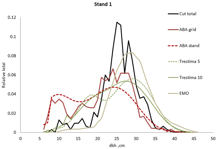
Fig. 1. Example of the breast height diameter (dbh) distributions for stand no. 1. EMO provided the best fit for total dbh distribution (all species together) according to Kolmogorov-Smirnov (KS) and Trestima 10 according to Error-Index (EI) goodness-of-fit tests.
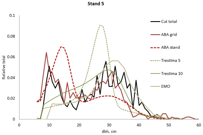
Fig. 2. Example of the breast height diameter (dbh) distributions for stand no. 5. ABA grid, Trestima 10 and EMO methods passed the Kolmogorov-Smirnov goodness-of-fit test while EMO had the best test values. Trestima 5 resulted in a too peaked dbh distribution.
Note that in terms of goodness-of-fit statistics, generally the best method was EMO and Trestima 10, which both requires a visit to the target stand.
In stand no. 1, EMO provided visually the best fit and was the only one that passed the KS test (Fig. 1). Trestima 10 followed slightly better the observed distribution than Trestima 5, especially when focusing on the largest dbh classes (Fig. 1). In stand no. 5, Trestima 5 showed excess kurtosis but, when all ten images were utilized in Trestima 10, the predicted distribution was one with the best fit (Fig. 2). The ABA grid reproduced the peaks and hollows of the observed distribution but the ABA stand resulted in a biased location for the peak for the smallest dbh classes and thus, generated the worst KS test values. Stand no. 7 had a decreasing, almost inverse J-shaped, dbh distribution. ABA grid and ABA stand were best at capturing the type of distribution (Fig. 3). The rejected case by Trestima 5 overestimated the proportion of the largest dbh classes but quite evenly distributed trees by Trestima 10 passed the KS test. Stand no. 6 was the easiest case to predict as each method passed the KS test. However, there were clear differences between predicted distributions. The observed dbh distribution was almost symmetric but with a slight bimodality due to the high proportion of the smallest dbh classes (Fig. 4). In terms of visual interpretation and according to KS and EI goodness-of-fit tests, Trestima 10 was the best. In this case, the peak by ABA grid methods did not coincide well with the peak of cut trees. The EMO generated distribution had an overabundance of trees with a DBH greater than 35 cm.
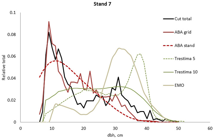
Fig. 3. Example of the breast height diameter (dbh) distributions for stand no. 7. ABA stand and ABA grid methods performed the best and second best according to Kolmogorov-Smirnov (KS) but according to Error-Index (EI), the ABA grid was slightly better. Trestima 5 and EMO did not pass the KS test and they provided the highest EI values.
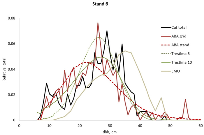
Fig. 4. Example of the breast height diameter (dbh) distributions for stand no. 6. Trestima 10 fitted the best according to Kolmogorov-Smirnov (KS) and Error-Index (EI) goodness-of-fit tests. The second best EI and KS test values were found using Trestima 5 and EMO, respectively. All the predicted dbh distributions passed the KS test.
3.4 Ranking of the applied methods
Ranking revealed two superior methods: Trestima 10 and ABA grid (Table 9). The strength of these methods is a superior goodness-of-fit of a predicted dbh distribution. Goodness of the distribution fit also resulted in good performance in standard stand and assortment characteristics, namely 9 and 7 times the least bias as well as 8 and 11 times the smallest RMSE.
| Table 9. Ranking the methods by the number of the best and the number of the worst cases among analysed criteria: Bias and RMSE for number of stems, basal area, basal area-weighted mean diameter, Lorey’s height, total volume, log and pulp wood volume by tree species and stand totals, as well as Kolmogorov-Smirnov (KS) and Error-Index (EI) tests. (Total of 70 criterion). The best performed method by each criteria is highlighted in bold. | ||||||||||
| Rank | Best | Worst | ||||||||
| Criteria | ABA grid | ABA stand | Trestima 5 | Trestima 10 | EMO | ABA grid | ABA stand | Trestima 5 | Trestima 10 | EMO |
| Bias | 9 | 3 | 7 | 7 | 2 | 2 | 4 | 4 | 2 | 15 |
| RMSE | 8 | 1 | 0 | 11 | 8 | 2 | 5 | 8 | 1 | 12 |
| KS | 1 | 0 | 0 | 2 | 4 | 1 | 1 | 5 | 0 | 0 |
| EI | 2 | 0 | 0 | 3 | 2 | 0 | 2 | 3 | 0 | 2 |
| Total | 20 | 4 | 7 | 23 | 16 | 5 | 12 | 20 | 3 | 30 |
The advantage of the Trestima 10 method was especially clear in the predicted number of stems, basal area and volume of the Norway spruce and broadleaves admixtures (see Table 3 and 4). The Trestima application, however, proved to be quite sensitive to the number of photos in the analysis. Applying 5 images often resulted in the worst test criterion (Table 9). Still, Trestima 5 had a total of 7 times the smallest bias. Note that a sample of 5 images was sufficient to reach 10% standard error in basal area in only two stands (Supplementary file 1).
Also the EMO application proved sensitive to a small number of sample trees. Namely the basal area of a stand is divided into tree species according to measured sample trees (six nearest trees per sample plot). EMO provided the best test criterion16 times (out of 70), but simultaneously, it frequently provided the worst criterion (30 times). EMO performed well with a dominating Scots pine stratum, but typically generated the worst test criteria for Norway spruce and birch admixtures (see Tables 4 to 7).
4 Discussion
The aim of this study was to assess and compare the accuracy of three pre-harvest inventory methods in predicting the dbh-height distribution of clear-cut stands. Of the applied methods, Trestima and EMO inventories require stand-specific samples but ABA does not require any stand-specific field measurements for prediction. The estimates of dbh and height distributions based on these methods were compared to accurate tree taper data measured and registered by the harvester measurement systems during the final cut. Finally, the accuracy of the prediction method is dependent on the generated individual trees – how alike or unlike they are compared with the observed trees and how alike they are distributed. The example given for the ABA grid method for stand 3 showed a remarkable similarity between modelled and cut tree dimensions (see Supplementary file 2).
In ABA, we used RF to select NN. In our study, RF was chosen based upon the quality of the results in previous studies and desirable statistical characteristics (i.e., the capability to predict multiple-response variables simultaneously, to use a large number of predictors without the problem of overfitting and to evaluate the accuracy with built-in functionality). The use of RF in NN estimation of forest variables has been common (Hudak et al. 2008; Yu et al. 2011; Vastaranta et al. 2013, 2014). For example, Hudak et al. (2008) demonstrated that the RF method is more robust and flexible for forest-variable prediction when compared to other NN distance measures, such as Euclidian distance, Mahalanobis distance or canonical-correlation analysis. In our NN predictions, the number of neighbours was set to one to keep the original variance in the data (Hudak et al. 2008). ABA results were generally in line or slightly worse than in other ABA studies carried out in the same study area (Holopainen et al. 2010; Yu et al. 2010; Vastaranta et al. 2013). Vastaranta et al. (2013) predicted G, DG, HG, and total volume with RMSEs of 17.8%, 19.1%, 7.8% and 17.9%, respectively. Especially the differences in the accuracy of basal area and total volume were obvious compared to our study and they could be explained partly from 5% and 12% underestimations using the ABA grid method, while those of Vastaranta et al. (2013) were only 0.3–0.4%. On the other hand, DG by the ABA grid method was even better (RMSE 11.0%) in the present study. It should be pointed out that our results were validated in limited mature forest conditions (7 mature stands) whereas a whole range of forest conditions (500 sample plots; D from 10 to 60 cm) were used in Vastaranta et al. (2013). It is typical in remote sensing- based inventories that stand characteristics in densely stocked stands are underestimated (Vastaranta et al. 2013). Holopainen et al. (2010) used ABA for predicting dbh distribution and timber assortments. Their results were validated with harvester-measured tree data from 12 clear-cutting sites. With ABA they obtained RMSEs of 79.2%, 33.6% and 78.6%, for pine, spruce and birch saw logs, respectively. The respective RMSEs in our study were 42.2%, 106.2% and 111.2%. Thus, accuracy of the dominating tree species in our study was 42.2% (pine) as it was 33.6% (spruce) in study by Holopainen et al. (2010). The species composition varied more in our validation stands compared to the study by Holopainen et al. (2010), which limits an interpretation. Based on previous studies, it can be deduced that the accuracy of the predicted timber assortments is much lower than prediction accuracy of total volume (Peuhkurinen et al. 2008) that is often used when validating quality of the inventory. In general, low prediction accuracy of the species-specific stand characteristics is seen as weakness of the ABA (White et al. 2013). Accuracy of the species-specific stand characteristics correlates highly with the accuracy of the predicted timber assortments.
Note that Weibull distribution in some ALS studies in Finland (Maltamo et al. 2006; Peuhkurinen et al. 2007; Packalén and Maltamo 2008; Holopainen et al. 2010) has been based on an old model by either Mykkänen (1986) or Kilkki et al. (1989). These Weibull models are not capable in predicting the smallest dbh classes resulting in serious underestimation in N. Nevertheless, as basal area-dbh distribution models they were relevant for predicting total and log wood volume (Siipilehto 1999; Maltamo et al. 2006). Inaccuracy in smallest diameters is due to modelling data – NFI based sample plots including trees selected with basal area factor 2. More accurate dbh distribution models exist (Kangas et al. 2007; Siipilehto et al. 2007) and here, we applied a parameter recovery method (Peuhkurinen et al. 2011). The advantage of parameter recovery is that it does not involve any additional errors in the used stand characteristics (Mehtätalo et al. 2007; Siipilehto and Mehtätalo 2013). Thus, stand characteristics interpreted for each grid could be fully utilized for solving the Weibull distribution. However, due to small 16 m × 16 m grid area we preferred random sampling when selecting dbh from the solved distribution.
It should be taken into account that Trestima and EMO applications required observations (photos or sample trees) from the target stands that are not needed in ABA. On the other hand, ABA is typically carried out at 10-year intervals and for large-areas at once (inventoried areas can vary from 50 000 ha to 1 million ha with the same scanning parameters, field plots, etc.). The current price of the ALS data is around 0.3€ per ha whereas the price of the field inventory is few euros per ha. In Finland, forest owners can access forest resource information collected using ABA for free. In our study, we had ABA information just before the cutting, which is not always possible in practice. Trestima and EMO provide flexible options for collecting stand-specific information just before cutting, but the additional costs is an issue. The Trestima app was superior to EMO in generated stand characteristics for admixtures, whereas EMO was superior for Scots pine. Trestima seemed quite sensitive to the number of images, but users can follow the results and standard error in basal area in real time. If sequential sampling is presumed, the risk of having a sample that is inadequate for target accuracy can be sharply reduced. Some clear cut stands appeared quite heterogeneous and even with 10 images the 10% convergence in the standard error of basal area was not achieved. Further, if only five images were included into the analysis, basal area convergence was met only twice (Suppl. file 1). The EMO method generalized relatively small samples to characterize stand structure using kernel smoothing. In addition, EMO divides the species-specific characteristics based on the measured sample trees. Nevertheless, EMO was obviously the best when it comes to volume characteristics of Scots pine. Unfortunately, EMO performed poorly for minor admixtures. The small samples of the EMO method translated into difficulties with capturing the shape of the dbh distribution. This was shown in some of the largest error-index values by EMO method.
Trestima and ALS methods were the most reliable in predicting stand characteristics and dbh distribution of standing trees prior to harvesting. Both methods had their strengths and weaknesses. When ABA was applied at grid level, it provided at its best very accurate dbh distributions that were able to follow bimodal- or even multimodal-shaped distributions. This is a very useful feature in stands having heterogeneous structure. On the other hand, all remote sensing methods have difficulties in two- or multistoried stands or situations in which trees have a clustered spatial structure (Uuttera et al. 1998; Mehtätalo 2006; Peuhkurinen et al. 2007).
The Trestima method provides the most accurate stand characteristics for the whole stand but the applied Weibull smoothing lacks the ability to produce bimodal- or multimodal-shaped species-specific distributions. The EMO method had originally been developed for producing accurate diameter-height-quality distributions of mature Scots pine forests and comprises features that inevitably provide biased results for admixtures. The method could be improved by executing relascope sampling for each tree species separately and by measuring the dbh of each tree within the relascope sample.
From the compared methods ABA is the least expensive, the Trestima method is the second least expensive and the EMO method the most expensive. The stand-specific cruising takes from half an hour to one hour in a typical Finnish stand of a size ranging from 1–3 hectares. With the EMO method additional time has to be reserved for data input. It is difficult to determine how accurate the predictions of standing trees need to be after all. What is the threshold value of accuracy for making decisions resulting in more profitable wood allocation and conversion solutions? The final judgment of the accuracy required has to be based on analytical comparisons of costs and revenues related to these decisions (Eid et al. 2004; Mäkinen et al. 2012).
Alternatives for kNN area-based ALS approach is to estimate regression models for required stand characteristics and/or for dbh distribution directly from ALS canopy metrics (Næsset 2002; Gobakken and Næsset 2004; Suvanto et al. 2005; Uuttera et al. 2006; Maltamo et al. 2007; Magnussen et al. 2012) or single tree detection (Peuhkurinen et al. 2007; Kankare et al. 2015). Also, one option is to produce dbh distributions directly from the measured trees of the field plots (Packalén and Maltamo 2008; Peuhkurinen et al. 2008). In the latter case the same trees will be multiplied, whenever the same plot describes the grid. In the Trestima method, empirical dbh distributions produced from the interpreted trees included in the relascope samples are also available. Those species-specific distributions can be bi- or multimodal. However, we believe that smoothing the small sample of interpret trees improved the results. At least, the species-specific distributions of the ground truth data resembled more like unimodal, although often extremely skewed for Norway spruce. Trestima methods included an average of 40 and 76 interpret trees from 5 and 10 images, respectively. This amount corresponded to 7% and 13% of the total number of cut trees per stand (see Suppl. file 1). Kopakka (2015) found that Trestima underestimates individual tree dbh and thus, its empirical dbh distribution also underestimated mean dbh. Accordingly, in this study DG was systematically underestimated with Trestima methods resulting in underestimation in basal area, too. Vastaranta et al. (2015) instead found slight overestimation (0.8–1.4%) in the dbh of the individual median tree for pine and broadleaves but 3.1% underestimation for spruce, while tree height and stand basal area were underestimated using Trestima. Trestima is under continuous development work. Thus, we do not know if the version of the processing software was the same in these studies.
The study material may be regarded as rather homogenous in terms of stand maturity and stand size. The study stands were all mature Scots pine- or Norway spruce-dominated forests with a stand size varying from 0.7 to 2.0 ha. The stand sizes may be regarded as rather typical for southern Finland. The pre-harvest inventory methods (Trestima and EMO) tested and compared here comprise a system, where sampling and measurements are spatially distributed evenly within the whole stand. In the ALS grid method, the diameter distributions are constructed by summing the individual diameter distributions of each 16 m × 16 m grid within the stand instead. In this sense the best methods, the Trestima and the ABA grid methods, probably produce similarly good results also in larger stands. Actually, if we look, say, at RMSE of the total volume, it seemed to decrease along with increased stand size. This was probably due to a decreased proportion of the most uncertain boundary grids.
Acknowledgement
This collaborative work was jointly executed by the following research project: “Efficient wood procurement as a part of value chain” funded by the Natural Resource Institute Finland (Luke), “Varma” funded by the TEKES and FWR Oy, “Data to Intelligence” funded by the TEKES and the Finnish Bioeconomy Cluster; and the Academy of Finland project “Centre of Excellence in Laser Scanning Research” (CoE-LaSR). We also want to thank Koskinen Oy from co-operation.
References
Bailey R.L., Dell T.R. (1973). Quantifying diameter distributions with the Weibull function. Forest Science 19(2): 97–104.
Bitterlich W. (1984). The Relascope Idea. Relative Measurements in Forestry. Commonwealth Agricultural Bureaux, London, UK. p. 242.
Breiman L. (2001). Random forests. Machine Learning 45(1): 5–32. http://dx.doi.org/10.1023/A:1010933404324.
Cajander A.K. (1925). The theory of forest types. Acta Forestalia Fennica 29. 108 p.
Cao Q.V. (2004). Predicting parameters of a Weibull function for modeling diameter distribution. Forest Science 50(5): 682–685.
Crookston N.L., Finley A.O. (2008). yaImpute: an R package for kNN imputation. Journal of Statistical Software 23(10): 1–16. http://dx.doi.org/10.18637/jss.v023.i10.
Gobakken T., Næsset E. (2004). Estimation of diameter and basal area distributions in coniferous forest by means of airborne laser scanner data. Scandinavian Journal of Forest Research 19: 529–542. http://dx.doi.org/10.1080/02827580410019454.
Gove J.H., Patil G.P. (1998). Modeling the basal area-size distribution of forest stand: a compatible approach. Forest Science 44(2): 285–297.
Haara A., Korhonen. K.T. (2004). Kuvioittaisen arvioinnin luotettavuus. Metsätieteen aikakauskirja 4/2004: 489–508. [In Finnish].
Holopainen M., Vastaranta M., Rasinmäki J., Kalliovirta J., Mäkinen A., Haapanen R., Melkas T., Yu X., Hyyppä J. (2010). Uncertainty in timber assortment estimates predicted from forest inventory data. European Journal of Forest Research 129: 1131–1142. http://dx.doi.org/10.1007/s10342-010-0401-4.
Holopainen M., Vastaranta M., Hyyppä J. (2014). Outlook for the next generation’s precision forestry in Finland. Forests 5(7): 1682–1694. http://dx.doi.org/10.3390/f5071682.
Hudak A.T., Crookston N.L., Evans J.S., Hall D.E., Falkowski M.J. (2008). Nearest neighbor imputation of species-level, plot-scale forest structure attributes from LiDAR data. Remote Sensing of Environment 112(5): 2232–2245. http://dx.doi.org/10.1016/j.rse.2007.10.009.
Hyyppä J., Hyyppä H., Yu X., Kaartinen H., Kukko H., Holopainen M. (2009). Forest inventory using small-footprint airborne lidar. In: Shan J., Toth C. (eds.). Topographic laser ranging and scanning: principles and processing. CRC Press, Taylor & Francis London. p. 335–370.
Järnstedt J., Pekkarinen A., Tuominen S., Ginzler C., Holopainen M., Viitala R. (2012). Forest variable estimation using a high-resolution digital surface model. ISPRS Journal of Photogrammetry and Remote Sensing 74: 78 – 84. http://dx.doi.org/10.1016/j.isprsjprs.2012.08.006.
Kangas A., Mehtätalo L., Maltamo M. (2007). Modelling percentile based basal area weighted diameter distribution. Silva Fennica 41(3): 425–440. http://dx.doi.org/10.14214/sf.282.
Kankare V., Liang X., Vastaranta M., Yu X., Holopainen M., Hyyppä M. (2015). Diameter distribution estimation with laser scanning based multisource single tree inventory. ISPRS Journal of Photogrammetry and Remote Sensing 108: 161–171. http://dx.doi.org/10.1016/j.isprsjprs.2015.07.007.
Kilkki P., Maltamo M., Mykkänen R., Päivinen R. (1989). Use of the Weibull function in the estimation the basal area dbh-distribution. Silva Fennica 23(4): 311–318. http://dx.doi.org/10.14214/sf.a15550.
Kopakka V.-M. (2015). Trestima älypuhelin kuvauksessa tunnistettujen puiden oikeellisuus. Ammattikorkeakoulun opinnäytetyö. Metsätalouden koulutusohjelma. Evo. 20 p. [In Finnish].
Korpunen H., Paltakari J. (2013). Testing an activity-based costing model with a virtual paper mill. Nordic Pulp and Paper Research Journal 28(1): 146–155. http://dx.doi.org/10.3183/NPPRJ-2013-28-01-p146-155.
Korpunen H., Mochan S., Uusitalo J. (2010). An activity-based costing method for sawmilling. Forest Products Journal 60(5): 420–431. http://dx.doi.org/10.13073/0015-7473-60.5.420.
Laasasenaho J. (1982). Taper curve and volume functions for pine, spruce and birch. Communicationes Instituti Forestalis Fenniae 108. 74 p.
Magnussen S., Næsset E., Gobakken T., Frazer G. (2012). A fine-scale model for area-based predictions of tree-size-related attributes derived from LiDAR canopy heights. Scandinavian Journal of Forest Research 27(3): 312–322. http://dx.doi.org/10.1080/02827581.2011.624116.
Mäkinen A., Kangas A., Nurmi M. (2012). Using cost-plus-loss analysis to define optimal forest inventory interval and forest inventory accuracy. Silva Fennica 46(2): 211 – 226. http://dx.doi.org/10.14214/sf.55.
Maltamo M., Puumalainen J., Päivinen R. (1995). Comparison of beta and Weibull functions for modelling basal area diameter distribution in stands of Pinus sylvestris and Picea abies. Scandinavian Journal of Forest Research 10: 284–295. http://dx.doi.org/10.1080/02827589509382895.
Maltamo M., Eerikäinen K., Packalén P., Hyyppä J. (2006). Estimation of stem volume using laser scanning-based canopy height metrics. Forestry 79(2): 217–229. http://dx.doi.org/10.1093/forestry/cpl007.
Maltamo M., Suvanto A., Packalén P. (2007). Comparison of basal area and stem frequency diameter distribution modelling using airborne laser scanner data and calibration estimation. Forest Ecology and Management 247: 26–34. http://dx.doi.org/10.1016/j.foreco.2007.04.031.
Mehtätalo L. (2005). Height-diameter models for Scots pine and birch in Finland. Silva Fennica 39(1): 55–66. http://dx.doi.org/10.14214/sf.395.
Mehtätalo L. (2006). Eliminating the effect of overlapping crowns from aerial inventory estimates. Canadian Journal of Forest Research 36: 1649–1660. http://dx.doi.org/10.1139/x06-066.
Mehtätalo L., Maltamo M., Packalen P. (2007). Recovering plot-specific diameter distribution and height-diameter curve using ALS based stand characteristics. International archives of photogrammetry, remote sensing and spatial information sciences 36(3/W52): 288–293. Proceedings of the ISPRS Workshop ‘Laser Scanning 2007 and SilviLaser 2007’ Espoo, September 12–14, Finland.
Mykkänen R. (1986). Weibull-funktion käyttö puuston läpimittajakauman estimoinnissa. Metsätalouden syventävien opintojen tutkielma, Joensuun yliopisto. 80 p. [In Finnish].
Næsset E. (2002). Predicting forest stand characteristics with airborne scanning laser using a practical two-stage procedure and field data. Remote Sensing of Environment 80: 88–99. http://dx.doi.org/10.1016/S0034-4257(01)00290-5.
Næsset E., Gobakken T., Holmgren J., Hyyppä H. Hyyppä J., Maltamo M., Nilsson M., Olsson H., Persson Å., Söderman U. (2004). Laser scanning of forest resources: the Nordic experience. Scandinavian Journal of Forest Research 1(4): 493–502. http://dx.doi.org/10.1080/02827580410019553.
Niemistö P., Korpunen H., Laurén A., Salomäki M., Uusitalo J. (2012). Impact and productivity of harvesting while retaining young understorey spruces in final cutting of downy birch. Silva Fennica 46(1): 81–97. http://dx.doi.org/10.14214/sf.67.
Nurminen T., Heinonen J. (2007). Characteristics and time consumption of timber trucking in Finland. Silva Fennica 41(3): 471–487. http://dx.doi.org/10.14214/sf.284.
Nurminen T., Korpunen H., Uusitalo J. (2006). Time consumption analysis of the mechanized cut-to-length harvesting system. Silva Fennica 40(2): 336–363. http://dx.doi.org/10.14214/sf.346.
Nurminen T., Korpunen H., Uusitalo J. (2009). Applying the activity-based costing to cut-to-length timber harvesting and trucking. Silva Fennica 43(5): 847–870. http://dx.doi.org/10.14214/sf.177.
Packalén P., Maltamo M. (2008). Estimation of species-specific diameter distributions using airborne laser scanning and aerial photographs. Canadian Journal of Forest Research 38(7): 1750–1760. http://dx.doi.org/10.1139/X08-037.
Peuhkurinen J., Maltamo M., Malinen J. (2007). Preharvest measurement of marked stands using airborne laser scanning. Forest Science 53(6): 653–661.
Peuhkurinen J., Maltamo M., Malinen J. (2008). Estimating species-specific diameter distributions and saw log recoveries of boreal forests from airborne laser scanning data and aerial photographs: a distribution-based approach. Silva Fennica 42(4): 625–641. http://dx.doi.org/10.14214/sf.237.
Peuhkurinen J., Mehtätalo L., Maltamo M. (2011). Comparing individual tree detection and the area-based statistical approach for retrieval of forest stand characteristics using airborne laser scanning in Scots pine stands. Canadian Journal of Forest Research 41(3): 583–598. http://dx.doi.org/10.1139/X10-223.
Päivinen R. (1980). On the estimation of stem diameter distribution and stand characteristics. Folia Forestalia 442. 28 p. [In Finnish with English summary].
PMP-ohje (1982). PMP-systeemin hoitokunta. [In Finnish].
Reynolds M.R, Burk T.E., Huang W.C. (1988). Goodness-of-fit tests and model selection procedures for diameter distribution models. Forest Science 34: 373–399.
Rouvinen T. (2014). Kuvia metsästä. Metsätieteen aikakauskirja 2/2014: 119–122. [In Finnish].
Schreuder H.T., Hafley W.L. (1977). A useful bivarite distribution for describing dtand dtructure of tree heights and diameters. Biometrics 33(3): 471–478. http://dx.doi.org/10.2307/2529361.
Siipilehto J. (1999). Improving the accuracy of predicted basal-area diameter distribution in advanced stands by determining stem number. Silva Fennica 33(4): 281–301. http://dx.doi.org/10.14214/sf.650.
Siipilehto J. (2000). A comparison of two parameter prediction methods for stand structure in Finland. Silva Fennica 34(4): 331–349. http://dx.doi.org/10.14214/sf.617.
Siipilehto J. (2011). Methods and applications for improving parameter prediction models for stand structures in Finland. Dissertationes Forestales 124. 56 p. http://dx.doi.org/10.14214/df.124.
Siipilehto J., Kangas A. (2015). Näslundin pituuskäyrä ja siihen perustuvia malleja läpimitta-pituus riippuvuudesta suomalaisissa talousmetsissä. Metsätieteen aikakauskirja 4/2015. [In Finnish].
Siipilehto J., Mehtätalo L. (2013). Parameter recovery vs. parameter prediction for the Weibull distribution validated for Scots pine stands in Finland. Silva Fennica 47(4): 1–22. http://dx.doi.org/10.14214/sf.1057.
Siipilehto J. Sarkkola S., Mehtätalo L. (2007). Comparing regression estimation techniques when predicting diameter distributions of Scots pine on drained peatlands. Silva Fennica 41(1): 333–349. http://dx.doi.org/10.14214/sf.300.
Sokal R.R., Rohlf F.J. (1981). Biometry. The principles and practice of statistics in biological research. W.H. Freeman and Company, San Francisco. 843 p.
StanForD. (2007). Standard for forest data and communication. Skogforsk. 10 p.
Suomen metsäkeskus (2014). Metsävaratiedon laatuseloste. http://www.metsakeskus.fi/sites/default/files/metsavaratiedon_laatuseloste.pdf. [In Finnish]. [Cited 2 Dec 2015].
Suvanto A., Maltamo M., Packalén, P, Kangas J. (2005). Kuviokohtaisten puustotunnusten ennustaminen laserkeilauksella. Metsätieteen aikakauskirja 4/2005: 413–428. [In Finnish].
Tham Å. (1988). Structure of Mixed Picea abies (L.) Karst. and Betula pendula Roth and Betula pubescens Ehrh. stands in South and middle Sweden. Scandinavian Journal of Forest Research 3(1–4): 355–369. http://dx.doi.org/10.1080/02827588809382523.
Trestima (2015). Forest inventory system v.1.1. 16 p.
Uusitalo J. (1997). Pre-harvest measurement of pine stands for sawing production planning. Acta Forestalia Fennica 259. 56 p.
Uusitalo J., Kivinen V.-P. (1998). Constructing bivariate dbh/dead branch height distribution of pines for use in sawing production planning. Scandinavian Journal of Forest Research 13(1–4): 509–514. http://dx.doi.org/10.1080/02827589809383012.
Uusitalo J., Kivinen V.-P. (2000). EMO: a pre-harvest measurement tool for predicting forest composition. In: Wood properties for industrial use. Measuring of wood properties, grades and qualities in the conversion chains and global wood chain optimisation. Proceedings of 3rd Workshop on COST Action E10, Espoo, Finland, June 19–20. p. 173–180.
Uuttera J., Haara A., Tokola T., Maltamo M. (1998). Determination of the spatial distribution of trees from digital aerial photographs. Forest Ecology and management 110(1–3): 275–282. http://dx.doi.org/10.1016/S0378-1127(98)00292-8.
Uuttera J., Anttila P., Suvanto A., Maltamo M. (2006). Yksityismetsien metsävaratiedon keruuseen soveltuvilla kaukokartoitusmenetelmillä estimoitujen puustotunnusten luotettavuus. Metsätieteen aikakauskirja 4/2006: 507–519. [In Finnish].
Varjo J. (1995). Latvan hukkaosan pituusmallit männylle, kuuselle ja koivulle metsurimittausta varten. In: Verkasalo E. (ed.). Puutavaran mittauksen kehittämistutkimuksia 1989–93. Metsäntutkimuksen tiedonantoja 558: 21–23. [In Finnish].
Vastaranta M., Wulder M.A., White J., Pekkarinen A., Tuominen S., Ginzler C., Kankare V., Holopainen M., Hyyppä J., Hyyppä H. (2013). Airborne laser scanning and digital stereo imagery measures of forest structure: comparative results and implications to forest mapping and inventory update. Canadian Journal of Remote Sensing 39(5): 382–395. http://dx.doi.org/10.5589/m13-046.
Vastaranta M., Saarinen N., Kankare V., Holopainen M., Kaartinen H., Hyyppä J., Hyyppä H. (2014). Multisource single-tree inventory in the prediction of tree quality variables and logging recoveries. Remote Sensing 6(4): 3475–3491. http://dx.doi.org/10.3390/rs6043475.
Vastaranta M., Gonzalez Latorre E., Luoma V., Saarinen N., Holopainen M., Hyyppä J. (2015). Evaluation of a smartphone app for forest sample plot measurements. Forests 6(4): 1179–1194. http://dx.doi.org/10.3390/f6041179.
Wang M., Rennolls K. (2007). Bivariate distribution modelling with tree diameter and height data. Forest Science 53(1): 16–24.
White J.C., Wulder M.A., Varhola A., Vastaranta M., Coops N.C., Cook B.D., Pitt D., Woods M. (2013). A best practices guide for generating forest inventory attributes from airborne laser scanning data using an area-based approach. Forestry Chronicle 89: 722–723. http://dx.doi.org/10.5558/tfc2013-132.
Yu X., Hyyppä J., Vastaranta M., Holopainen M., Viitala R. (2011). Predicting individual tree attributes from airborne laser point clouds based on the random forests technique. ISPRS Journal of Photogrammetry and Remote Sensing 66(1): 28 – 37. http://dx.doi.org/10.1016/j.isprsjprs.2010.08.003.
Total of 69 references.
