Lauri Haataja  ,
Ville Kankaanhuhta,
Timo Saksa
,
Ville Kankaanhuhta,
Timo Saksa
Reliability of self-control method in the management of non-industrial private forests
Haataja L., Kankaanhuhta V., Saksa T. (2018). Reliability of self-control method in the management of non-industrial private forests. Silva Fennica vol. 52 no. 1 article id 1665. https://doi.org/10.14214/sf.1665
Highlights
- Self-control method was found reliable at the main stages of the forest regeneration process
- Only slight overestimation was found in self-control results of soil preparation and planting and small underestimation in self-control of young stand management
- Diverse utilizing of self-control data is possible in support of service providers operations.
Abstract
This study seeks to determine the extent to which self-control data can be relied upon in the management of private forests. Self-control (SC) requires the forest workers to evaluate their own work quality to ensure the clients’ needs are met in terms of soil preparation, planting and young stand management. Self-control data were compared to an independent evaluation of the same worksites. Each dataset had a hierarchical structure (e.g., sample plot, regeneration area and contractor), and key quality indicators (i.e., number of prepared mounds, planted seedlings or crop trees) were measured for each plot. Self-control and independent-assessments (IA) were analyzed by fitting a multi-level multivariate model containing explanatory variables. No significant differences were observed in terms of soil preparation (number of mounds) or young stand management (number of crop trees) between self-control and independent-assessments. However, the self-control planting data included a slight but significant overestimation of the number of planted seedlings. Discrepancies are discussed in terms of sampling error and other explanatory factors. According to overall results, self-control methods are reliable at every stage of the forest regeneration process. As such, the diverse utilizing of self-control data is possible in support of service providers operations.
Keywords
forest management;
soil preparation;
quality control;
young stand management;
forest regeneration;
boreal silviculture;
forest planting
-
Haataja,
Natural Resources Institute Finland (Luke), Natural resources, Juntintie 154, FI-77600 Suonenjoki, Finland
E-mail
lauritapiohaataja@gmail.com
- Kankaanhuhta, Natural Resources Institute Finland (Luke), Natural resources, Juntintie 154, FI-77600 Suonenjoki, Finland E-mail ville.kankaanhuhta@luke.fi
- Saksa, Natural Resources Institute Finland (Luke), Natural resources, Juntintie 154, FI-77600 Suonenjoki, Finland E-mail timo.saksa@luke.fi
Received 19 June 2016 Accepted 3 January 2018 Published 23 January 2018
Views 115756
Available at https://doi.org/10.14214/sf.1665 | Download PDF

1 Introduction
According to a recent inventory of Finnish forests, the quality of young forest stands has decreased. Only 45% of young seedling stands, 29% of advanced seedling stands and 20% of young thinning stand were good in quality (Statistical Yearbook of Forestry 2014). This poses a serious threat to their development and long-term commercial viability, especially given that Finnish forestry aims to significantly increase the demand for forest-based bioproducts in the near future (Finnish Government 2015). In order to maintain and improve sustainability, the amount of high-quality young forest stands should be increased. Quality management of the whole regeneration chain is one promising solution for this challenge.
Organizing cost-effective and reliable quality control in primary production industries (e.g., forestry) is challenging. According to EU legislation, quality control of the food production industry has relied on a system of self-control (SC). The Finnish Food Safety Authority (Evira) requires producers to arrange and perform systematic SCs that address the risks associated with cold-chain management and storage for example. The format of the SC is based on operator capacity and nature of the work involved and focus on steps where risk of failure is greatest and where external process controls are complex and expensive (Finnish Food… 2016). In forest services quality management is based on free markets, where customer satisfaction through quality standards and certification is the goal. In this context the SC is a relevant tool, respectively.
In forestry, the annual workload takes place over a wide area during a narrow period of time, making it difficult and expensive to supervise and ensure that it is performed to a uniform and high standard. Although different companies have relied on various quality control systems (Kalland 2002), Finnish forestry has gradually shifted from external monitoring to SC of forest workers performing the various operations in forest regeneration and management (i.e., soil preparation, planting, cleaning and young stand management).
From the worker’s viewpoint, SC begins with the operation and desired result agreed by the worker, employer and client according to worksite conditions and other circumstances. By agreeing on a target quality, the forest worker knows what they are being asked to do (Gryna 2001). Through SC, forest workers systematically evaluate the quality of their work and compare it to a set of target standards. If necessary, the quality is improved ensuring the desired result (Deming 1986; Juran and Godfrey 1998). Self-control provides a system by which work quality can be monitored in real-time and responses made rapidly and cost-effectively to unexpected developments at the worksite.
In chain-oriented silvicultural services, mistakes done at the earlier stages of chain tend to appear pronouncedly at the later stages of chain. Consequently, resources must be aimed for repairing the mistakes. Thus, quality control is a preventative action and it profits each party of silvicultural operations. Self-control data can also be used to inform and integrate workers and suppliers involved in subsequent operations. For example, SC of soil preparation provides the number of prepared spots which determine the number of seedlings required for planting. Given that work quality is an important factor at every step in the forest regeneration process (Gitlow 2001; Lillrank 2010; Luoranen et al. 2012), it is critical to know the extent to which SC data are reliable, consistent and to understand the factors that influence their collection in order to improve the protocol and, consequently, the regeneration and management of future forests.
The quality of each step in the regeneration process can be evaluated according to several critical success factors (CSFs) of sub-processes. These CSFs are the focus of SC protocols, and help the worker tailor their work strategy in order to meet the target (Gryna 1988). For example, the number of prepared spots is the main CSF in soil preparation because it provides the foundation for planting and future performance of the seedling. High quality sites are for instance characterized by approximately 2000 mounds ha–1 that are large enough for planters to plant seedlings correctly but not so large as to provide substrate for opportunistic broadleaf trees (Uotila et al. 2010). Planting work is evaluated in terms of the proportion of seedlings that are planted correctly, i.e., stems anchored well in the soil and their roots reaching nutritious humus layer when possible (Long 1991; Luoranen and Viiri 2016). Seedlings should also be planted in the centre of the prepared spot, maximizing the distance from the humus edge and thereby minimizing the risk of pine weevil (Hylobius abietis) attack (Heiskanen and Viiri 2005) and competition with adjacent vegetation (Örlander et al. 1990). The main activity involved in the management of young stands is to thin the stand to a suitable density and composition in which the remaining crop trees can grow quickly and unhindered (Harstela 2007) (Table 1).
| Table 1. Quality factors and predictors to be measured in the main stages of forest regeneration. | |
| Stage | Quality factors and predictors to be measured |
| Soil preparation | Number of prepared spots ha–1 |
| Length, width and height of prepared spot (cm) | |
| Soil type (coarse – fine – peat) | |
| Stoniness (yes – no) | |
| Logging debris (yes – no) | |
| Planting | Number of planted seedlings ha–1 |
| Planting depth (cm) | |
| Seedlings distance from unprepared soil (cm) | |
| Seedling anchor (yes – no) | |
| Young stand management | Number of crop trees ha–1 |
| Composition of stand (number of pines, spruces and birches) | |
| Stand height, average (m) | |
| Stand diameter, average (cm) | |
| Number of stumps ha–1 | |
| Stump diameter, average (cm) | |
Earlier studies of forestry management have shown that monitoring itself has a positive impact on work quality (Kalland 2002; Harstela et al. 2006; Kankaanhuhta et al. 2010) but, as yet, little is known about the performance or influence of SC in this context. Given the increasing popularity of SC among forestry organizations, it is important to appreciate its functionality, efficiency and reliability as the basis of quality control.
The aim of this study is to estimate the reliability of SC data at each step in the forest regeneration process, i.e., from soil preparation to young stand management in non-industrial private forests. Data used in this study were generated through SC protocols developed and tested by seven silviculture service providers operating in privately-owned boreal forests in Southern Finland (Haataja et al. 2014). The accuracy and reliability of SC were analyzed by comparing SC data to control inventories, which were used as independent-assessment (IA) data.
2 Material and methods
2.1 Framework
The seven service providers in this case study were five Forest Owners Associations and two private forest companies providing services for non-industrial private forests (NIPF) in Southern Finland. Organization culture and adaption rate for quality management differed between these service providers. Human resource management and remuneration of workers varied also between service providers. In this study, the purpose was to obtain and explore specific variation in this business.
During 2011–2014, three service providers operating in Northern Savonia and four operating in Southern Ostrobothnia completed SC protocols for work performed on a combined total of 5047 ha. Work quality was evaluated by forest workers as part of the operation and as the work took place. Approximately 9% of this total (211 sites; ca. 432 ha) was evaluated through SC by the workers responsible as well as an independent evaluation by Finnish Forest Research Institute (FFRI) personnel (Table 2). Independent-assessment was conducted on soil preparation sites processed by 16 forest workers, planting sites (28 workers), and management of young stands (19 workers). Eighty-five percent of sites were processed by a single worker and the remaining 15% by two or more workers working as a team. The final evaluations were made in autumn 2014 (Fig. 1).
| Table 2. Number of independent-assessment sites according to service provider, stage of chain and year. | ||||
| Variable | Soil preparation | Planting | Young stand management | Total |
| Service provider | ||||
| 1 | 27 | 16 | 10 | 53 |
| 2 | 59 | 21 | 16 | 96 |
| 3 | 1 | - | 2 | 3 |
| 4 | 7 | 20 | 4 | 31 |
| 5 | - | 7 | 13 | 20 |
| 6 | - | 4 | - | 4 |
| 7 | - | - | 4 | 4 |
| Total | 94 | 68 | 49 | 211 |
| Year | ||||
| 2011 | 6 | - | 3 | 9 |
| 2012 | 35 | 24 | 33 | 92 |
| 2013 | 33 | 35 | 4 | 72 |
| 2014 | 20 | 9 | 9 | 38 |
| Total | 94 | 68 | 49 | 211 |
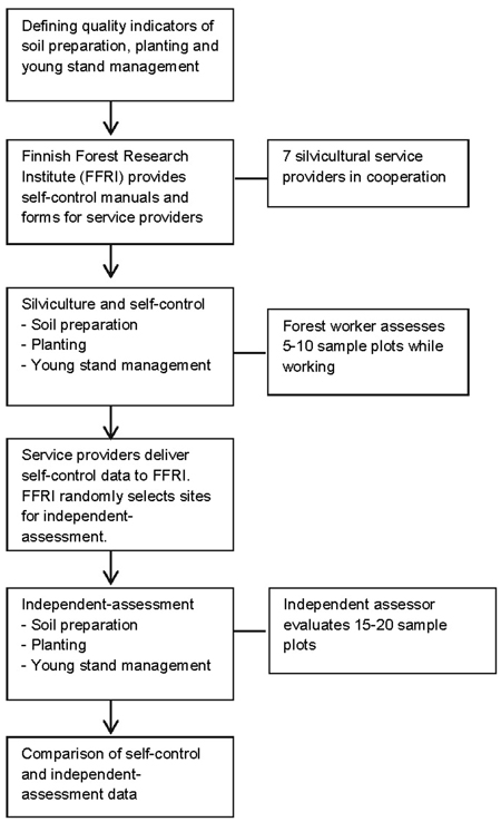
Fig. 1. Schematic of the study design and sequence.
2.2 Evaluation protocols
2.2.1 Self-control (SC)
In SC, the individual performing the work was responsible for the evaluation of 5–10 sample plots depending on site area (Table 3). .For soil preparation and young stand management sites, sample plots were determined according to the following sampling routine at the site. First, the forest worker estimated the duration of the work required for the site and then divided this by the number of sample plots to be evaluated. Thus, the worker generated a work-evaluation schedule that completed the work as well as the evaluations for the required number of sample plots within the allotted period. Alternatively, the forest worker could generate a schedule in terms of a fuel estimate, i.e., by dividing the number of fuel-tank refills by the number of sample plots in young stand management.
| Table 3. Number of sample plots to be measured in self-control. | |
| Regeneration area (ha) | Number of sample plots |
| 0.50 – 1.99 | 5 |
| 2.00 – 3.99 | 6 |
| 4.00 – 5.99 | 7 |
| 6.00 – 7.99 | 8 |
| 8.00 – 9.99 | 9 |
| 10 or bigger | 10 |
At planting worksites, the work-evaluation sampling was based on the number of seedlings to be planted divided by the number of sample plots to be measured at the site. For example, if the site was 2.7 ha due to receive 5400 seedlings (2000 per ha), a sample plot would be evaluated after every 900th seedling planted (= six seedling trays) to yield six sample plots (5400/6 = 900).
In each worksite sample plots were determined by sweeping a full circle with a 3.99 m rod (forming a plot area of ca. 50 m2). For soil preparation sites, only mounds and patches that occurred within the sample plot and which had been prepared to an acceptable quality were counted. Every other borderline case was counted out. The mound closest to the center of a sample plot was scrutinized more carefully and its approximate dimensions (width, length and height) were determined to within 5 cm. Soil texture type was defined with a three-class scale: 1. coarse mineral; 2. fine mineral (grain size < 0.06 mm); 3. peat. Stoniness and logging debris were scored “yes” or “no” depending on the extent to which they hindered soil preparation.
In planting sites, the number of seedlings planted inside a sample plot was counted. Seedlings planted in mounds and seedlings planted in unprepared soil were counted separately. Planting depth was measured to the nearest cm for the seedling planted closest to the plot center. The minimum distance of the same seedling from the humus edge was also measured to the nearest 5 cm and the quality of its planting determined in terms of its anchor in the soil.
For sites receiving young stand management, tree species were identified and counted separately within each sample plot. A median tree of the dominant tree species was scrutinized more closely and its height was estimated with the help of a 3.99 m rod and its diameter at breast height was determined with a tape measure. Cut stumps were counted within 1.78 m radius of the plot center, and an average stump diameter was calculated with tape measure based on five stumps closest to the plot center. The number of stumps was not applied as quality indicator. This data was used for pricing of services and in application for silvicultural subsidies.
Finnish Forest Research Institute provided self-control manuals and forms for service providers and trained their foremen (Fig. 1). The implementation of measurements was at the responsibility of service providers. Each worker passed their completed evaluation forms to their manager and from there to the FFRI.
2.2.2 Independent-assessment (IA)
Self-control sites were randomly selected for independent-assessment, wherein a grid of sample plots was created covering the whole site encompassing 15 sample plots on sites smaller than 2 ha or 20 sample plots on sites of 2 ha or larger. Exact centers of sample plots were objectively determined with a measuring device and compass. Sample plots were oriented along the cardinal points (or intercardinal points when more appropriate) to form a regular grid. As in SC, IA sample plots were delimited for all worksites and activities by sweeping a full circle with a 3.99 m rod (plot area ca. 50 m2). At challenging sites a pole was secured to the ground in the center and the sample plot was defined by a 3.99 m cable tied to it. The same set of variables was evaluated in IA and SC.
2.3 Description of assessment data
The IA data of soil preparation work was collected on 94 sites (180 ha; 1501 sample plots) processed during 2012–2014 in seven different municipalities. At these sites, soil preparation work was carried out by four different service providers during 2011–2014. The SC dataset consisted of 510 sample plots (Table 4). Soil preparation was carried out with different mounding methods according to prevalent conditions: ca. 93% of sites received mostly spot mounding (i.e., upturned humus forming a flat mound with a double humus layer); ditch mounding dominated at 6% of sites and 1% had equal amounts of spot and ditch mounds (Table 5). The most common soil type was coarse mineral (ca. 50% of sites). Stoniness and logging debris were perceived to be a work hindrance in 11% and 3% of sites, respectively. The mean number of mounds in a sample plot was 9.1 (IA) and 9.9 (SC) (Table 6).
| Table 4. Description of self-control (SC) and independent-assessment (IA) datasets in each stage. | ||||||
| Variable | No. of sites | Area (ha) | Sample plots | |||
| N | Min (per site) | Max (per site) | Mean (per site) | |||
| Soil preparation | ||||||
| SC | 94 | 180 | 510 | 2 | 10 | 5.4 |
| IA | 94 | 180 | 1501 | 4 | 23 | 16.4 |
| Planting | ||||||
| SC | 68 | 153 | 376 | 2 | 15 | 5.5 |
| IA | 68 | 153 | 1111 | 2 | 27 | 16.3 |
| Young stand management | ||||||
| SC | 49 | 99 | 276 | 2 | 12 | 5.7 |
| IA | 49 | 99 | 658 | 3 | 21 | 14.6 |
| Table 5. Main characteristics of soil preparation sites in independent-assessment. | |||||
| Class variable | No. of sites | % of sites | Area (ha) | No. of sample plots | % of sample plots |
| Soil type | |||||
| Coarse mineral | 48 | 51.1 | 84 | 748 | 49.8 |
| Fine mineral | 33 | 35.1 | 62 | 509 | 33.9 |
| Peat | 7 | 7.4 | 15 | 183 | 12.2 |
| No dominant | 6 | 6.4 | 19 | - | - |
| Unknown | 61 | 4.1 | |||
| Stony soil | 10 | 10.6 | 16 | 98 | 6.6 |
| Disruptive logging debris | 3 | 3.2 | 4 | 72 | 4.9 |
| Soil preparation | |||||
| Spot mounding | 87 | 92.6 | 160 | 1295 | 86.3 |
| Ditch mounding | 6 | 6.3 | 17 | 188 | 12.5 |
| Patching | - | - | - | 12 | 0.8 |
| No dominant | 1 | 1.1 | 3 | 6 | 0.4 |
| Site type (*) | |||||
| OMaT | - | - | - | - | - |
| OMT | 16 | 17 | 22 | 255 | 17 |
| MT | 52 | 55.3 | 102 | 859 | 57.2 |
| VT | 8 | 8.5 | 20 | 118 | 7.9 |
| CT | - | - | - | - | - |
| CIT | - | - | - | - | - |
| No dominant | 3 | 3.2 | 5 | - | - |
| Unknown | 15 | 16 | 31 | 269 | 17.9 |
| Target density | |||||
| 1600 | 1 | 1.1 | 1.4 | 20 | 1.3 |
| 1800 | 16 | 17 | 32.7 | 269 | 17.9 |
| 1900 | 8 | 8.5 | 19.2 | 122 | 8.1 |
| 2000 | 36 | 38.3 | 53.3 | 537 | 35.8 |
| Unknown | 33 | 35.1 | 73.2 | 553 | 36.8 |
| Soil preparation equipment | |||||
| Mounding plate | 50 | 53.2 | 88 | 766 | 54 |
| Digger shovel | 31 | 33 | 70 | 514 | 34.3 |
| Both | 8 | 8.5 | 11 | 132 | 8.8 |
| Unknown | 5 | 5.3 | 11 | 89 | 5.9 |
| Work period | |||||
| Spring | 53 | 56.4 | 103 | 838 | 55.8 |
| Autumn | 40 | 42.5 | 76 | 643 | 42.8 |
| Unknown | 1 | 1.1 | 1 | 20 | 1.3 |
| (*) Site type according to Cajander (1949). | |||||
| Table 6. Main characteristics of modelling data set for soil preparation. | ||||||
| Variable | N | Mean | SD | Min | Max | |
| Self-control 2011–2014 | ||||||
| No. of spot mounds | 510 | 8.40 | 3.67 | 0 | 20 | |
| No. of ditch mounds | 510 | 1.21 | 3.23 | 0 | 17 | |
| No. of inverted mounds | 510 | 0.05 | 0.67 | 0 | 11 | |
| No. of patches | 510 | 0.24 | 1.21 | 0 | 11 | |
| No. of preparation spots | 510 | 9.90 | 1.73 | 6 | 20 | |
| Height of mound, cm | 446 | 16.82 | 5.32 | 9 | 35 | |
| Footprint preparation spot, m2 | 468 | 0.37 | 0.13 | 0.05 | 0.9 | |
| Independent-assessment 2012–2014 | ||||||
| No. of spot mounds | 1501 | 7.9 | 3.59 | 0 | 18 | |
| No. of ditch mounds | 1501 | 1.1 | 2.83 | 0 | 16 | |
| No. of inverted mounds | 1501 | 0.0 | 0.00 | 0 | 0 | |
| No. of patches | 1501 | 0.1 | 0.67 | 0 | 11 | |
| No. of preparation spots | 1501 | 9.1 | 2.18 | 1 | 18 | |
| Height of mound, cm | 1478 | 16.7 | 6.30 | 5 | 60 | |
| Footprint of preparation spot, m2 | 1501 | 0.5 | 0.29 | 0.07 | 2.56 | |
| N = number of sample plots. Note: variation among N occurs due to the removal of incomplete or illogical measurements. | ||||||
Independent-assessments took place in 2012–2014 at 68 planting sites (153 ha; 1111 sample plots) processed by six different service providers operating in eight different municipalities. Plantings were performed 2012–2014, and the SC dataset represents 376 sample plots processed by 28 forest workers (Table 4). Most (93%) planting sites were prepared with mounding, with the remainder being stump lifted (4%) or disc-trenched areas (3%) (Table 7). The dominant species planted were Norway spruce (Picea abies (L.) Karst.: 85%) and Scots pine (Pinus sylvestris L.: 15%). The mean number of seedlings planted per plot was 9.0 (IA) and 10.0 (SC) (Table 8).
| Table 7. Main characteristics of planting sites in independent-assessment. | |||||
| Class variable | No. of sites | % of sites | Area (ha) | No. of sample plots | % of sample plots |
| Seedling | |||||
| Pine | 8 | 11.8 | 13.6 | 162 | 14.6 |
| Spruce | 52 | 76.5 | 120.1 | 949 | 85.4 |
| Pine + spruce | 8 | 11.8 | 19.2 | ||
| Soil preparation | |||||
| Mounding | 63 | 92.6 | 136.5 | 1023 | 92 |
| Disc trenching | 2 | 2.9 | 1.6 | 28 | 2.5 |
| Stump removal | 3 | 4.4 | 14.8 | 60 | 5.5 |
| Target density | |||||
| 1800 | 17 | 25 | 44.4 | 300 | 27 |
| 1900 | 1 | 1.5 | 1.1 | 15 | 1.4 |
| 2000 | 37 | 54.4 | 71.9 | 560 | 50.4 |
| Unknown | 13 | 19.1 | 35.5 | 236 | 21.2 |
| Site type (*) | |||||
| OMaT | - | - | - | - | - |
| OMT | 11 | 16.2 | 27.2 | 192 | 17.3 |
| MT | 28 | 41.2 | 55.2 | 483 | 43.5 |
| VT | 13 | 19.1 | 26.3 | 210 | 18.9 |
| CT | - | - | - | - | - |
| CIT | - | - | - | - | - |
| Unknown | 16 | 23.5 | 44.2 | 226 | 20.3 |
| (*) Site type according to Cajander (1949). | |||||
| Table 8. Main characteristics of modelling data set for planting. | |||||
| Variable | N | Mean | SD | Min | Max |
| Self-control 2011–2014 | |||||
| No. of seedlings planted to prepared spot | 376 | 9.51 | 2.19 | 0 | 15 |
| No. of seedlings planted to unprepared soil | 376 | 0.49 | 1.25 | 0 | 9 |
| No. of seedlings planted overall | 376 | 10.00 | 1.58 | 4 | 15 |
| Planting depth, cm | 371 | 4.58 | 1.41 | 1 | 10 |
| Distance from humus edge, cm | 289 | 32.78 | 16.86 | 0 | 130 |
| Independent-assessment 2012–2014 | |||||
| No. of seedlings planted to prepared spot | 1111 | 8.09 | 2.61 | 0 | 18 |
| No. of seedlings planted to unprepared soil | 1111 | 0.95 | 1.87 | 0 | 13 |
| No. of seedlings planted overall | 1111 | 9.03 | 2.37 | 0 | 22 |
| Planting depth, cm | 1111 | 6.21 | 2.38 | 0 | 10 |
| Distance from humus edge, cm | 1073 | 23.45 | 13.28 | 0 | 70 |
| N = number of sample plots. Note: variation among N occurs due to the removal of incomplete or illogical measurements. | |||||
The IA dataset for young stand management was collected 2012–2014 and represents 49 sites (99 ha; 658 sample plots) processed by six service providers operating in eight municipalities. The SC dataset consists of 276 sample plots processed 2011–2014 by 19 forest workers (Table 4). Scots pine was the dominant tree at 40%, Norway spruce at 28%, birch (Betula spp.) at 16% of sites (Table 9). The composition of tree species was approximately equal at 16% of sites. The mean number of crop trees per plot was 10.7 (IA) and 10.3 (SC). The mean number of cut trees (i.e., stumps) was 15.0 (IA) and 24.2 (SC) (Table 10).
| Table 9. Main characteristics of young stand management sites in independent-assessment. | |||||
| Class variable | No. of stands | % of stands | Area (ha) | No. of sample plots | % of sample plots |
| Site type (*) | |||||
| OMaT | - | - | - | - | - |
| OMT | 6 | 12.2 | 13.5 | 82 | 12.5 |
| MT | 11 | 22.4 | 21.5 | 175 | 26.6 |
| VT | 6 | 12.2 | 11.5 | 102 | 15.5 |
| CT | - | - | - | 11 | 1.7 |
| CIT | - | - | - | - | - |
| No dominant | 1 | 2 | 1.2 | - | - |
| Unknown | 25 | 51 | 51.1 | 288 | 43.8 |
| Dominant tree | |||||
| Pine | 19 | 38.8 | 45.3 | 276 | 41.9 |
| Spruce | 14 | 28.6 | 30.7 | 189 | 28.7 |
| Birch | 8 | 16.3 | 10 | 143 | 21.7 |
| No dominant | 8 | 16.3 | 12.8 | 50 | 7.6 |
| Method | |||||
| Early clearing | 7 | 14.3 | 17.8 | 85 | 12.9 |
| Normal tending | 35 | 71.4 | 72.9 | 428 | 65 |
| Later tending | 7 | 14.3 | 8.1 | 145 | 22 |
| (*) Site type according to Cajander (1949). | |||||
| Table 10. Main characteristics of modelling data set for young stand management. | |||||
| Variable | N | Mean | SD | Min | Max |
| Self-control 2011–2014 | |||||
| No. of spruces | 276 | 3.29 | 3.63 | 0 | 11 |
| No. of pines | 276 | 4.57 | 5.14 | 0 | 16 |
| No. of birches | 276 | 2.49 | 2.91 | 0 | 11 |
| No. of other broadleaf trees | 276 | 0.00 | 0.00 | 0 | 0 |
| No. of trees overall | 276 | 10.34 | 2.21 | 3 | 16 |
| Dominant height of trees, m | 276 | 4.43 | 1.73 | 2 | 10 |
| Diameter of trees, cm | 276 | 5.04 | 2.23 | 2 | 13 |
| No. of stumps | 276 | 24.18 | 13.21 | 0 | 69 |
| Diameter of stumps, cm | 225 | 3.08 | 1.06 | 1 | 6 |
| Independent-assessment 2012–2014 | |||||
| No. of spruces | 658 | 3.27 | 3.78 | 0 | 16 |
| No. of pines | 658 | 4.67 | 4.94 | 0 | 20 |
| No. of birches | 658 | 2.78 | 3.29 | 0 | 18 |
| No. of other broadleaf trees | 658 | 0.02 | 0.16 | 0 | 2 |
| No. of trees overall | 658 | 10.74 | 3.21 | 2 | 25 |
| Dominant height of trees, m | 658 | 5.00 | 2.27 | 2 | 15 |
| Diameter of trees, cm | 658 | 5.10 | 2.44 | 1 | 13 |
| No. of stumps | 649 | 15.07 | 12.26 | 0 | 100 |
| Diameter of stumps, cm | 635 | 2.48 | 1.11 | 0.5 | 8.5 |
| N = number of sample plots. Note: variation among N occurs due to the removal of incomplete or illogical measurement. | |||||
2.4 Multivariate multilevel analysis of the assessment data
Differences between the paired SC and IA datasets were studied by fitting a normally-distributed multivariate multilevel model for each operation (i.e., preparation, planting, young stand management) (Miina and Saksa 2006; Kankaanhuhta and Saksa 2013). By using a multivariate multilevel model, it is possible to utilize the covariance among different response variables to generate more accurate parameter estimates and the resulting statistical inference. The data had three hierarchy levels in soil preparation and planting, and two levels in young stand management. In soil preparation, the hierarchy consisted of sample plots within regeneration area within combined machine contractor and year; note that the machine contractor could have more than one worker operating a machine. In planting, the hierarchy contained sample plots within regeneration area within worker. In young stand management, the hierarchy contained sample plots within stand.
With respect to soil preparation and planting, the comparison of SC and IA data was made by modeling normally-distributed multivariate multilevel models:
![]()
In the soil preparation model, subscripts i, j, and k refer to sample plot, regeneration area and combined contractor and year, respectively. In the planting model, i, j, and k refer to sample plot, regeneration area and worker. The multivariate model for soil preparation consisted of three response variables, which were estimated simultaneously: number; size (m2), and; height (cm) of mounds. Response variables in the multivariate model for planting were number of planted seedlings, planting depth (cm) and distance from humus edge (cm). In the young stand management multivariate multilevel model, crop trees and cut trees were modeled separately due to the different purposes of these indicators. In both young stand management models, i and j refer to sample plot and stand:
![]()
Response variables in the multivariate model for crop trees were: number of coniferous trees; number of birches; height of trees (m), and; diameter of trees (cm). In the multivariate model for cut trees, the response variables were: number of stumps, and; average diameter of stumps (cm).
Categorical predictors treated in the soil preparation models were stoniness, soil type and logging debris. In the planting model, the predictor was tree species and the crop tree model for young stand management was without predictors. In the cut-tree model, the predictor was dominant tree species. All models were estimated simultaneously by applying the Restricted Iterative Generalized Least Squares (RIGLS) algorithm in MLwiN 2.34 software (Rasbash et al. 2015). Candidate models were compared and evaluated by means of a likelihood ratio test using the χ2 distribution. The most common variable classes recorded were used as reference classes. For each operation, IA data were used as a reference class as the number of sample plots was approximately three times higher than for the corresponding SC data. The dominant soil type at soil preparation sites was coarse mineral. At planting sites, the dominant tree species was spruce. Independent-assessment data were used as a reference class in the crop tree model without other predictors. In the cut-trees model, pine as a dominant tree was used as a reference class.
The error variances of SC were calculated for contractor, planting worker and stand levels through a covariance matrix of SC and IA data. This was not possible at the sample plot level since the location of plots within each stand varied.
3 Results
3.1 Density as the main quality indicator
3.1.1 Soil preparation
At the regeneration area level, the average number of mounds/hectare was 1982 (SD = 302) in SC and 1829 (SD = 280) in IA (Fig. 2). In 68% of cases, the SC data suggested the density of soil preparation spots was higher than the value recorded in the IA (Fig. 3a). The correlation between measurements was 0.40 (Pearson). If we accept ±20% as a permissible level of discrepancy between the SC and IA datasets, 72% of cases fell within this range. If we limit the tolerance to ±10% discrepancy, 48% of cases fall within limits.
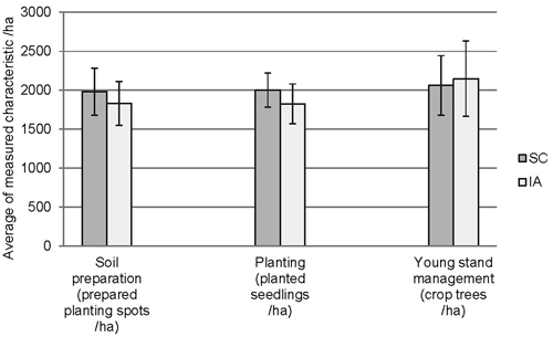
Fig. 2. Means and standard deviations of the assessed variables in different stages of the regeneration process (SC = Self-control, IA = Independent assessment).
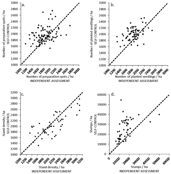
Fig. 3. Comparison of self-control and independent-assessment results. Each point of the scatter plot displays individual working site.
3.1.2 Planting
The average number of planted seedlings per ha was 2002 (SD = 221) in SC and 1825 (SD = 256) in IA (Fig. 2). In 78% of cases, the number of planted seedlings per ha was higher in the SC data (Fig. 3b). The correlation between measurements was 0.54 (Pearson). Seventy-eight percent of cases fell within a tolerance of ±20%, 44% at a tolerance of ±10%.
3.1.3 Young stand management
The mean density of crop trees was 2062 (SD = 383) trees ha–1 in SC and 2148 (SD = 483) trees ha–1 in IA (Fig. 2). The crop tree density was higher for the IA data in 65% of cases (Fig. 3c). Correlation between measurements was 0.76 (Pearson). Eighty-two percent of cases fell within a tolerance of ±20% and 59% within ±10% tolerance. The mean number of cut trees was 25341 (SD = 10701) stumps ha–1 in SC and 15989 (SD = 7880) stumps ha–1 in IA. In 87% of cases, the SC recorded more stumps than IA (Fig. 3d). Correlation between measurements was 0.49 (Pearson).
3.2 Factors influencing reliability
3.2.1 Soil preparation
When analyzing variation in soil preparation through multivariate multilevel modeling, the reference class used was the IA observation for a coarse soil, where stoniness or logging debris was not considered to be a hindrance to work efficiency (Table 11).
| Table 11. Multivariate multilevel model for soil preparation. Parameter estimates and variance components of equations for number, height and footprint of prepared spots. The most common values of the class variables were used as a reference class. | |||||||||||
| Predictor | No. of prepared spots | Height of mound (cm) | Footprint of prepared spot (m2) | ||||||||
| Estimate | SE | χ2-value | Estimate | SE | χ2-value | Estimate | SE | χ2-value | |||
| Intercept | 9.76 | 0.29 | 1103.3 *** | 16.16 | 0.50 | 1053.8 *** | 0.56 | 0.04 | 235.9 *** | ||
| Discrepancy | 0.55 | 0.34 | 2.6 ns | –0.68 | 1.03 | 0.4 ns | –0.18 | 0.04 | 19.1 *** | ||
| Soil texture | |||||||||||
| Fine mineral | |||||||||||
| IA | 0.13 | 0.14 | 0.9 ns | 0.60 | 0.45 | 1.8 ns | 0.00 | 0.02 | 0.1 ns | ||
| SC | 0.00 | 0.24 | 1.55 | 0.77 | 4.0 ** | 0.01 | 0.02 | 0.3 ns | |||
| Peat | |||||||||||
| IA | –0.59 | 0.18 | 11.1 *** | 1.92 | 0.58 | 10.9 *** | –0.02 | 0.02 | 0.8 ns | ||
| SC | 0.46 | 0.28 | 2.7 * | 2.57 | 0.90 | 8.3 ** | 0.07 | 0.03 | 6.9 ** | ||
| Stony soil | |||||||||||
| IA | –1.92 | 0.21 | 86.9 *** | –0.97 | 0.70 | 1.9 ns | –0.06 | 0.03 | 5.2 * | ||
| SC | 1.04 | 0.27 | 14.3 *** | –0.12 | 0.90 | 0.0 ns | 0.02 | 0.03 | 0.7 ns | ||
| Logging debris | |||||||||||
| IA | –1.82 | 0.21 | 72.9 *** | –2.08 | 0.74 | 7.9 ** | –0.04 | 0.03 | 2.7 ns | ||
| SC | 1.16 | 0.28 | 16.9 *** | 0.81 | 0.97 | 0.7 ns | 0.02 | 0.03 | 0.4 ns | ||
| Random part | |||||||||||
| SD (uk) | |||||||||||
| IA | 1.05 | 0.4721 | - | 1.41 | 1.1733 | - | 0.12 | 0.0071 | - | ||
| SC | 0.81 | 0.3097 | - | 3.26 | 4.667 | - | 0.08 | 0.0027 | - | ||
| SD (ukj) | |||||||||||
| IA | 0.78 | 0.1276 | - | 2.01 | 0.9953 | - | 0.15 | 0.0041 | - | ||
| SC | 0.68 | 0.1149 | - | 2.11 | 1.138 | - | 0.04 | 0.0005 | - | ||
| SD (ekji) | |||||||||||
| IA | 1.65 | 0.1032 | - | 5.79 | 1.2801 | - | 0.20 | 0.0016 | - | ||
| SC | 1.06 | 0.0826 | - | 3.12 | 0.765 | - | 0.08 | 0.0005 | - | ||
| Discrepancy = difference between self-control (SC) and independent-assessment (IA), SE = Standard error, SD = Standard deviation. * significant at 0.05, ** significant at 0.01 and *** significant at 0.001 level. “ns” = non-significant at 0.1 level. Subscripts i, j and k refer to sample plot, regeneration area and combined contractor and year. | |||||||||||
The IA intercept for soil preparation was 9.76, or an average of 1952 (9.76 × 200) mounds ha–1. Correspondingly, SC value was 100 mounds ha–1 higher, which in practice meant 0.5 mounds per sample plot. Contractor accounted for 25% of variation (Table 12). Respectively, the standard deviation of SC error was 214 (![]() × 200) mounds ha–1. At the regeneration area level, the standard deviation of the error was 169 mounds ha–1. Stony soil and logging debris significantly reduced the number of mounds ha–1 in the IA. Soil texture had a negative and highly significant effect in IA in case of peat lands.
× 200) mounds ha–1. At the regeneration area level, the standard deviation of the error was 169 mounds ha–1. Stony soil and logging debris significantly reduced the number of mounds ha–1 in the IA. Soil texture had a negative and highly significant effect in IA in case of peat lands.
| Table 12. Multivariate multilevel model for soil preparation. Variance explained at different hierarchical levels for number, height and footprint of prepared spots. Fixed effects are the same as in Table 11. | ||||||||||
| Variable and hierarchy level | Variance | Proportion % | Error variance of self-control | Correlation r | Error proportion % | |||||
| Without fixed effects | With fixed effects | Difference % | Without fixed effects | With fixed effects | Without fixed effects | With fixed effects | Difference % | |||
| No. of prepared spots | ||||||||||
| Contractor | 1.104 | 1.100 | 0.4 | 22.2 | 24.8 | 1.51 | 1.15 | 23.8 | –0.71 | 105 |
| Regeneration area | 0.886 | 0.615 | 30.6 | 17.8 | 13.9 | 1.03 | 0.71 | 31.3 | –0.65 | 115 |
| Sample plot | 2.992 | 2.720 | 9.1 | 60.1 | 61.3 | - | - | - | - | - |
| Mound height (cm) | ||||||||||
| Contractor | 1.754 | 1.982 | –13.0 | 4.4 | 5.0 | 17.19 | 10.38 | 39.6 | –0.19 | 523 |
| Regeneration area | 4.047 | 4.058 | –0.3 | 10.1 | 10.3 | 5.46 | 4.21 | 23.0 | –0.46 | 104 |
| Sample plot | 34.106 | 33.468 | 1.9 | 85.5 | 84.7 | - | - | - | - | - |
| Footprint of prepared spot (m2) | ||||||||||
| Contractor | 0.022 | 0.014 | 38.4 | 25.1 | 17.6 | 0.03 | 0.02 | 37.2 | –0.80 | 121 |
| Regeneration area | 0.024 | 0.023 | 2.5 | 26.5 | 29.5 | 0.03 | 0.03 | –3.6 | –0.96 | 112 |
| Sample plot | 0.043 | 0.042 | 3.9 | 48.4 | 52.9 | - | - | - | - | - |
The intercept estimate for mound height was 16 cm (Table 11). In SC, mounds were on average slightly smaller (0.7 cm). Contractor accounted for only 5% of variation in IA and regeneration area for 10% (Table 12). At the contractor level, the error associated with SC was large but the standard deviation was about 3 cm (![]() ). Mounds were taller on fine mineral and peat soils in both assessments, but not significant in the IA of mounds on fine mineral soils. Logging debris significantly lowered the average height of mounds in the IA.
). Mounds were taller on fine mineral and peat soils in both assessments, but not significant in the IA of mounds on fine mineral soils. Logging debris significantly lowered the average height of mounds in the IA.
The reference estimate for mound size in the IA was 0.56 m2, i.e., a 75 × 75 cm footprint. In SC, mounds were one third smaller, respectively a 60 × 60 cm footprint. Thirty and 18% of the variation in the IA data was explained by regeneration area and contractor, respectively. The standard deviation of SC error was 0.17 and 0.14 m2 at the regeneration area and contractor levels, respectively. Mounds formed on peat soil were significantly larger in the SC data. Stoniness was significantly associated with a reduction of mound size in the IA data.
With respect to soil preparation (i.e., mounding), more of the variation within and among scored variables was explained by sample plot rather than regeneration area or contractor (Table 12).
3.2.2 Planting
The reference tree species used in the multivariate multilevel model for planting was Norway spruce (Table 13). The mean number of planted seedlings was 1776 ha–1 (8.88 × 200). In SC, an additional 158 (0.79 × 200) seedlings ha–1 were planted than suggested by the IA. Regeneration area and worker accounted for 14% and 12% of the variation in IA, respectively (Table 14).
| Table 13. Multivariate multilevel model for planting. Parameter estimates and variance components of the equations for the number of planted seedlings, planting depth, and distance from humus edge. The most common values of the class variables were used as a reference class. | |||||||||||
| Predictor | Planted seedlings | Planting depth (cm) | Distance from humus (cm) | ||||||||
| Estimate | SE | χ2-value | Estimate | SE | χ2-value | Estimate | SE | χ2-value | |||
| Intercept | 8.88 | 0.23 | 1520.8 *** | 6.32 | 0.31 | 416.6 *** | 23.11 | 1.60 | 209.3 *** | ||
| Discrepancy | 0.79 | 0.21 | 14.01 *** | –1.63 | 0.32 | 26.2 *** | 8.94 | 3.16 | 8.0 ** | ||
| Seedling species | |||||||||||
| Pine | |||||||||||
| IA | 0.40 | 0.31 | 1.65 ns | 0.19 | 0.30 | 0.4 ns | –1.65 | 1.84 | 0.8 ns | ||
| SC | 0.08 | 0.33 | 0.06 ns | –1.48 | 0.36 | 16.9 *** | 4.23 | 3.76 | 1.3 ns | ||
| Mixed | |||||||||||
| IA | 1.07 | 0.58 | 3.38 ns | –0.28 | 0.65 | 0.2 ns | 0.00 | 0.00 | 0.0 | ||
| SC | 0.00 | 0.00 | 0.00 | 0.00 | 0.00 | 0.0 | 0.00 | 0.00 | 0.0 | ||
| Random part | |||||||||||
| SD (uk) | |||||||||||
| IA | 0.83 | 0.3385 | - | 1.30 | 0.6402 | - | 6.21 | 16.5823 | - | ||
| SC | 0.95 | 0.33 | - | 0.80 | 0.2557 | - | 11.64 | 54.0982 | - | ||
| SD (ukj) | |||||||||||
| IA | 0.91 | 0.2303 | - | 0.91 | 0.2185 | - | 5.59 | 8.2111 | - | ||
| SC | 0.39 | 0.0954 | - | 0.49 | 0.0904 | - | 4.29 | 10.7414 | - | ||
| SD (ekji) | |||||||||||
| IA | 2.07 | 0.1884 | - | 1.83 | 0.1472 | - | 10.81 | 5.2042 | - | ||
| SC | 1.25 | 0.1273 | - | 0.95 | 0.0747 | - | 11.69 | 12.7362 | - | ||
| Discrepancy = difference between self-control (SC) and independent-assessment (IA). SE = Standard error, SD = Standard deviation. * significant at 0.05, ** significant at 0.01 and *** significant at 0.001 level. “ns” = non-significant at 0.1 level. Subscripts i, j and k refer to sample plot, regeneration area and worker. | |||||||||||
| Table 14. Multivariate multilevel model for planting. Variances explained at different hierarchical levels for the number of planted seedlings, planting depth, and distance from humus edge. Fixed effects are the same as in Table 13. | ||||||||||
| Variable and hierarchy level | Variance | Proportion % | Error variance of self-control | Correlation r | Error proportion % | |||||
| Without fixed effects | With fixed effects | Difference % | Without fixed effects | With fixed effects | Without fixed effects | With fixed effects | Difference % | |||
| No. of planted seedlings | ||||||||||
| Worker + year | 0.835 | 0.690 | 17.4 | 14.1 | 11.8 | 0.42 | 0.52 | –24 | –0.26 | 75 |
| Regeneration area | 0.804 | 0.835 | –3.9 | 13.5 | 14.3 | 0.34 | 0.32 | 6 | –0.97 | 39 |
| Sample plot | 4.301 | 4.304 | –0.1 | 72.4 | 73.8 | - | - | - | - | - |
| Planting depth (cm) | ||||||||||
| Worker + year | 1.698 | 1.699 | 1.0 | 28.8 | 28.9 | 1.63 | 1.65 | –1 | –0.81 | 97 |
| Regeneration area | 0.834 | 0.821 | 1.9 | 14.2 | 14.0 | 0.92 | 0.69 | 25 | –0.84 | 84 |
| Sample plot | 3.358 | 3.361 | –0.2 | 57.0 | 57.1 | - | - | - | - | - |
| Distance from humus edge (cm) | ||||||||||
| Worker + year | 38.892 | 38.522 | –0.1 | 20.8 | 20.6 | 121.74 | 133.48 | –10 | –0.25 | 347 |
| Regeneration area | 31.891 | 31.270 | 1.6 | 17.0 | 16.8 | 69.02 | 62.65 | 9 | –0.85 | 200 |
| Sample plot | 116.575 | 116.808 | –0.1 | 62.2 | 62.6 | - | - | - | - | - |
The estimate of planting depth intercept was 6.3 cm. In SC, seedlings were 1.6 cm closer to the surface. Worker and regeneration area accounted for 29% and 14% of the variation in the IA data, respectively. At the worker level, the standard deviation of SC error was 1.3 cm (![]() ) and 0.8 cm at the regeneration area level. The SC data suggested pine seedlings were 1.5 cm closer to the surface.
) and 0.8 cm at the regeneration area level. The SC data suggested pine seedlings were 1.5 cm closer to the surface.
The mean distance of seedling from the humus edge was 23 cm. This distance was ca. 9 cm greater in the SC data. Worker and regeneration area accounted for 21% and 17% of the variation in IA, respectively. At the worker level, the standard deviation of SC error was 12 cm (![]() ) and 8 cm at the regeneration area level (Table 14). Relatively more of the variation in the planting assessment data was explained by sample plot than by regeneration area or worker (Table 14).
) and 8 cm at the regeneration area level (Table 14). Relatively more of the variation in the planting assessment data was explained by sample plot than by regeneration area or worker (Table 14).
3.2.3 Young stand management
Young stand management assessments do not appear to be correlated with stand characteristics (Table 15). The number of coniferous or deciduous trees did not differ between assessments. The mean number of coniferous trees and birches left standing in IA was 1532 and 600 ha–1, respectively (Table 15). Self-control suggested 48 fewer coniferous trees and 44 fewer birches ha–1 than IA. Stand level accounted for 67% (coniferous trees) and 51% (birches) of the variation in the IA data (Table 16). At the stand level, the standard deviation of SC error was about 200 (![]() × 200) coniferous trees ha–1 and 89 (
× 200) coniferous trees ha–1 and 89 (![]() × 200) birches ha–1.
× 200) birches ha–1.
| Table 15. Multivariate multilevel model for young stand management (crop trees). Parameters, estimates and variance components of the equations for the number of coniferous trees, number of birches, height of trees, and diameter of trees. The most common values of the class variables were used as a reference class. | ||||||||||||
| Predictor | Number of coniferous trees | Number of birches | Average height of trees | Average diameter of trees | ||||||||
| Estimate | SE | χ2-value | Estimate | SE | χ2-value | Estimate | SE | χ2-value | Estimate | SE | χ2-value | |
| Intercept | 7.66 | 0.49 | 245.0 *** | 3.00 | 0.35 | 71.5 *** | 4.97 | 0.27 | 334.2 *** | 5.05 | 0.27 | 338.1 *** |
| Discrepancy | –0.24 | 0.23 | 1.1 ns | –0.22 | 0.16 | 1.9 ns | –0.57 | 0.14 | 16.7 *** | –0.09 | 0.15 | 0.4 ns |
| Random part | ||||||||||||
| SD (uj) | ||||||||||||
| IA | 3.33 | 2.3722 | - | 2.38 | 1.2422 | - | 1.87 | 0.7329 | - | 1.87 | 0.7455 | - |
| SC | 3.19 | 2.2295 | - | 2.23 | 1.1465 | - | 1.39 | 0.4267 | - | 1.68 | 0.6365 | - |
| SD (uji) | ||||||||||||
| IA | 2.35 | 0.3152 | - | 2.35 | 0.3152 | - | 1.18 | 0.0802 | - | 1.42 | 0.1158 | - |
| SC | 2.13 | 0.423 | - | 1.94 | 0.3515 | - | 0.99 | 0.0913 | - | 1.27 | 0.1512 | - |
| Discrepancy = difference between self-control (SC) and independent-assessment (IA). SE = Standard error, SD = Standard deviation. * significant at 0.05, ** significant at 0.01 and *** significant at 0.001 level. “ns” = non-significant at 0.1 level. Subscripts i and j refer to sample plot and stand. | ||||||||||||
| Table 16. Multivariate multilevel model for young stand management (crop trees). Variances explained at different hierarchical levels for number of coniferous trees, number of birches, height of trees, and diameter of trees. The fixed effects are the same as in Table 15. | ||||||||||
| Variable and hierarchy level | Variance | Proportion % | Error variance of self-control | Correlation r | Error proportion % | |||||
| Without fixed effects | With fixed effects | Difference % | Without fixed effects | With fixed effects | Without fixed effects | With fixed effects | Difference % | |||
| Number of coniferus trees | ||||||||||
| Stand | 11.115 | - | - | 66.9 | - | 1.04 | - | - | –0.30 | 9 |
| Sample plot | 5.507 | - | - | 33.1 | - | - | - | - | - | - |
| Number of birches | ||||||||||
| Stand | 5.676 | - | - | 50.8 | - | 0.20 | - | - | –0.43 | 3 |
| Sample plot | 5.507 | - | - | 49.2 | - | - | - | - | - | - |
| Height of stand (m) | ||||||||||
| Stand | 3.513 | - | - | 63.5 | - | 0.69 | - | - | –0.44 | 20 |
| Sample plot | 2.023 | - | - | 36.5 | - | - | - | - | - | - |
| Average diameter of stand (cm) | ||||||||||
| Stand | 3.500 | - | - | 71.4 | - | 0.63 | - | - | –0.74 | 18 |
| Sample plot | 1.400 | - | - | 28.6 | - | - | - | - | - | - |
In IA, crop trees were on average 5 m tall with an average diameter of 5 cm at breast height. Trees, on average, were 0.57 m shorter in SC, but the diameters were practically the same. In the IA data, 64% of the variation in height, and 71% of the variation in diameter was explained by stand. At the stand level, the standard deviation of SC error was about 0.83 m (![]() ) for height, 0.79 cm (
) for height, 0.79 cm (![]() ) for diameter.
) for diameter.
The dominant tree species influenced results of the cut-tree model due to different target densities (Table 17). In general, dominance of spruce or birch was associated with an increase in the removal of trees compared to plots where pine was dominant. The number of cut stumps was higher in SC as was their average diameter. The number of cut trees per ha was 13 730 in IA and 21 336 in SC, with stand accounting for 28% of variation in the IA data (Table 18), and the standard deviation of SC error was about 7500 stumps ha–1 at the stand level. The average stump diameter was 2.4 cm (IA) and 3 cm (SC), with stand accounting for 27% of the variation in IA, and the standard deviation of SC error was 0.49 cm.
| Table 17. Multivariate multilevel model for young stand management (removed trees). Parameter estimates and variance components of the equations for number of stumps and average diameter of stumps. The most common values of the class variables were used as a reference class. | |||||||
| Predictor | Number of stumps | Average diameter of stumps (cm) | |||||
| Estimate | SE | χ2 -value | Estimate | SE | χ2 -value | ||
| Intercept | 13.73 | 1.30 | 112.3 *** | 2.4045 | 0.11 | 477.8 *** | |
| Discrepancy | 7.606 | 1.78 | 18.4 *** | 0.5604 | 0.15 | 14.9 *** | |
| Dominant tree | |||||||
| Spruce | |||||||
| IA | 3.41 | 1.57 | 4.7 * | 0.00 | 0.13 | 0.0 ns | |
| SC | 1.86 | 2.38 | 0.6 ns | 0.18 | 0.18 | 1.0 ns | |
| Birch | |||||||
| IA | 3.81 | 1.48 | 6.6 * | 0.17 | 0.13 | 1.9 ns | |
| SC | 3.59 | 2.40 | 2.2 ns | –0.12 | 0.19 | 0.4 ns | |
| Mixed | |||||||
| IA | 3.61 | 1.88 | 3.7 * | 0.25 | 0.16 | 2.3 ns | |
| SC | 5.12 | 4.16 | 1.5 ns | –0.37 | 0.36 | 1.1 ns | |
| Random part | |||||||
| SD (uj) | |||||||
| IA | 6.62 | 10.885 | - | 0.57 | 0.0811 | - | |
| SC | 9.08 | 20.0964 | - | 0.71 | 0.1347 | - | |
| SD (uji) | |||||||
| IA | 10.56 | 6.4266 | - | 0.94 | 0.0517 | - | |
| SC | 9.18 | 7.8922 | - | 0.75 | 0.0589 | - | |
| Discrepancy = difference between self-control (SC) and independent-assessment (IA). SE = Standard error, SD = Standard deviation. * significant at 0.05, ** significant at 0.01 and *** significant at 0.001 level. “ns” = non-significant at 0.1 level. Subscripts i and j refer to sample plot and stand. | |||||||
| Table 18. Multivariate multilevel model for young stand management (removed trees). Variances explained at different hierarchical levels for number of stumps and average diameter of stumps. The fixed effects are the same as in Table 17. | ||||||||||
| Variable and hierarchy level | Variance | Proportion % | Error variance of self-control | Correlation r | Error proportion % | |||||
| Without fixed effects | With fixed effects | Difference % | Without fixed effects | With fixed effects | Without fixed effects | With fixed effects | Difference % | |||
| No. of stumps | ||||||||||
| Stand | 44.68 | 43.76 | 2.1 | 28.5 | 28.2 | 55.55 | 56.27 | –1 | –0.18 | 129 |
| Sample plot | 112.13 | 111.48 | 0.6 | 71.5 | 71.8 | - | - | - | - | - |
| Average stump diameter (cm) | ||||||||||
| Stand | 0.33 | 0.32 | 2.9 | 27.3 | 26.7 | 0.22 | 0.24 | –9 | –0.10 | 76 |
| Sample plot | 0.89 | 0.89 | –0.1 | 72.7 | 73.3 | - | - | - | - | - |
3.2.4 Model fit
Fit of the multivariate models was explored by comparing their variances with and without significant fixed effects at each hierarchic level. In soil preparation, contractor explained 24.8% and 22% of the variation with and without fixed effects in the number of mounds prepared, respectively (Table 12). Combining contractor and regeneration area accounted for 38.7% (with: 24.8 + 13.9%) and 40% (without: 22.2 + 17.8%). Fixed effects clearly reduced the variance associated with the SC error.
In planting, worker accounted for 12% and 14% of the variation in the number of seedlings with and without fixed effects, respectively (Table 14). In combination, worker and regeneration area accounted for 26.1% (with: 11.8 + 14.3%) and 27.6% (without: 14.1 + 3.5%).
In young stand management, there were no fixed effects in the crop tree model (Table 16). The cut-tree model was run with and without fixed effects: at the regeneration area accounted for 28.2% (with) 28.5% (without) of the variation in the number of stumps (Table 18).
4 Discussion
In production industries, quality is usually measured according to general standards or case-specific goals. In this study, SC data were compared to an independent evaluation of the same work. Although the IA result is not a standard or agreed value, it can be considered as the best objective baseline available. Significant discrepancies were detected between the SC and IA datasets, suggesting a bias similar to the findings of similar studies (Shewhart 1931; Hintermaier 1951; Juran and Godfrey 1998).
The aim of this case study was to determine the extent to which SCs completed by forest workers are sufficiently objective and accurate to be considered reliable for management purposes. Since different types of service providers were included to this study, we expected variation among assessments and reliability among forest workers and contractors (Kempe 1995; Saksa and Kankaanhuhta 2007), and we sought understanding of variation and reasons for inaccuracies. Furthermore, the multilevel modelling applied supported this approach.
Discrepancies between SC and IA can be due to numerous sources; the most common concern sampling. Factors such as measurement technique, density and resolution determine how precisely the sample represents reality. The SC protocol calls for 5 to 10 objectively selected sample plots, while sampling in the IA was completed for 15 or 20 sample plots based on site area. In SC according to sampling routine the aim was to obtain as randomized sample as possible. However, it was possible that selection of sample plot locations in SC was either purposively or subjectively poorly implemented instead of randomization. Selection routine weighted by the consumption of working time might have influenced the selection of sample plot locations purposively. The worker might have also selected more representative sample plot locations in his view point.
In IA, systematic sampling desing was used. As such, the estimates provided by the IA data are expected to be more precise and accurate. While the influence of sampling (i.e., measurement) error decreases as sample size increases (Häggman 1997), sample density is a compromise between cost, time and required accuracy (Hämäläinen and Räsänen 1993; Kangas et al. 2004). In the SC, accuracy is a priority but the time spent for assessing and recording the quality of work has to be considered. However, it can be argued that this is money well spent as such activities are specifically designed to ensure high quality in a product or service (Feigenbaum 1991; Kondo and Kano 1998).
Other issues concern the size of a sample plot, how it is delimited, and where it is located. The IA sample plot was delimited mainly by a 3.99 m solid cable while measuring tools varied in SC. The most common tool used for defining plot in SC was 3.99 meter telescope rod. Too long or too short rod causes systematic error which can lead to a significant difference in result. When radius of plot is 3.99 meters, one measured soil preparing spot, seedling or tree inside plot relates to 200 items per hectare.
Discrepancies could also be due to subjective scoring of the quality variables (Ishikawa 1985). For example, SC of soil preparation requires the worker to count the number of mounds that are of a sufficient quality for planting, and standards may vary among workers. Additionally, mounds mistakenly counted outside the boundaries of the sample plot could inflate the mound density estimate, and there remains the concern that some workers have a tendency to over- or underestimate the quality of their work to avoid any negative consequences (Baker 1988).
Workers operating an excavator tended to slightly overestimate the number of mounds or patches (<1 mound per sample plot; not significant) they prepared with respect to the independent assessor. A slight overestimate is a logical and expected property of SC, a phenomenon also noted by Maalismaa (2015). Both assessments judged mound height similarly and multivariate modeling showed that different soil types had similar effects on this variable in both datasets. Mound footprint was larger in the IA data, a difference 0.18 m2 which translates to a 15 cm increase of the length and width of a mound over SC. This is partly due to changes in mound shape (i.e., spreading) between the SC and IA (Heiskanen et al. 2013). Furthermore, mound footprint is difficult to measure accurately as the edges are often indeterminate. Almost one third of the variation was explained by regeneration area, suggesting local factors influence this variable.
In planting, the forest worker had a tendency to estimate a slightly higher (<1 seedling per sample plot) seedling density than the independent assessor. Saksa and Kankaanhuhta (2007) found that assessments of seedling density by two different evaluators differed by more than 20% on a quarter of the sites assessed three years after planting. Their observations agree with the results of our study, as assessments of this variable differed by up to 20% in 22% of sites. The IA estimated that seedlings were deeper than in the SC. The discrepancy is significant, but the implication being that workers are underestimating the quality of this aspect of planting bodes well for the performance of the regenerated stand (Long 1991; Luoranen and Viiri 2016). However, planting depth is difficult to determine precisely and accurately. To measure the linear distance from the soil surface to the top of the seedling root ball would require the planting to be disturbed and thereby diminish subsequent seedling performance. Worker’s estimates of planting depth were particularly variable, emphasizing the measurement error associated with this aspect. Therefore, the modification of this quality indicator towards an acceptable threshold value may be considered. This threshold value should be adjusted according to the method of site preparation. The minimum distance from the humus edge to the planted seedling was significantly higher in the SC data, but this average and that of the IA were within the recommended range. This may be due to workers measuring the distance between a randomly-selected point on the humus edge rather than the minimum distance. In this case, the development of more precise SC guidelines and protocols may be considered.
Another factor to consider is that SCs were performed while the work was taking place while IAs were completed at some later time, e.g., the following year. Seasonal factors (e.g., winter snowpack, heavy rains, summer drought) can affect the evaluation of soil preparation and planting, and summer growth of the herb layer could distort an autumn estimate of seedling density.
In young stand management, one of the most likely sources of error concerns how small trees were counted to generate the estimate of tree density. In our study, trees were counted if they were at least half the mean height of the stand. Kankaanhuhta (2015) studied reliability in SC report of young stand management work in Finland, and our results generally agree in that while discrepancies were found, they were trivial. Kankaanhuhta (2015) found that, on average, SC reported 56 more coniferous trees ha–1 were left standing after young stand management than IA. We found a discrepancy of 48 trees ha–1 on average, but with IA estimating the higher density. Although the studies suggesting opposing trends with respect to this variable, discrepancy was minor in both studies. Tree height was generally measured as an estimate made relative to a 3.99 m rod, a technique that could suffer from measurement error especially in taller stands. Furthermore, trees had obviously grown in the period between assessments creating a directional bias in the IA.
In young stand management, the number of cut trees (i.e., stumps) was estimated to be much higher in SC. This could be explained by differences in sampling method that are due to minimizing labor costs. The assessment is based on the amount of time required to thin the site, and sample plots tend to be those where the worker spends the most time. This hypothesis was tested through simulation where estimates from the IA data were weighted by the time consumed calculated from Finnish collective agreement functions (TTS 2016). In these simulations, the standard deviations of measurement error were approx. 45% lower than those of the SC data. Consequently, SC sample plots are concentrated in dense parts of young stands, which accounts for the difference between the assessments. The SC estimate can also misrepresent the entire site where dense parts (e.g., along ditch edges) are unsuitable for crop trees and which can lower stand density. The discrepancy between IA and SC was the lowest when pine was the dominant tree species. Depending on the service concepts, remuneration and quality goals of the service provider, the counting and measurement of stumps maybe reconsidered.
According to our results, SC data is reliable at main stages of the forest regeneration process representing the key quality indicators. However, depending on the local circumstances, the key indicators of SC may be reconsidered or modified. Furthermore, independent and objective control measurements are recommendable to motivate the application of this tool. Ideally, SC provides an accurate account of the work performed and the site in general that can be forwarded to the forest owner as part of the invoice and guarantee offered by the service provider. We encourage the use of SC data in the updating and completion of forest resource information systems as well as for other analytical purposes. However, this requires service providers to continue SC programs as a means of quality control and tool to continuously improve their own operations.
Acknowledgements
The research was conducted in co-operation with volunteering Forest Owners Associations, two private forest companies, Finnish Forest Centre and Finnish Forest Research Institute. The research group is grateful for all previously mentioned. Furthermore, we are most grateful for Dr. Juha Lappi for valuable advice on the statistical analysis. We also thank Lauri Herlevi and Jouni Hurskainen for their important contribution to the independent-assessment data collecting and coding. In addition, we thank Kyösti Sipilä for the comments on evaluation protocols. We also thank Lucidia and Dr Michael Hardman for revising the English language.
References
Baker E. (1988). Managing human performance. In: Juran J., Gryna F. (eds.). Juran’s quality control handbook. 4th ed. McGraw-Hill, New York. p. 10.1–10.61.
Cajander A.K. (1949). Forest types and their significance. Acta Forestalia Fennica 56. 71p. https://doi.org/10.14214/aff.7396.
Deming W.E. (1986). Out of the crisis. MIT Center for Advanced Engineering Study. 507 p.
Feigenbaum A. (1991). Total quality control. 3rd. rev. ed. McGraw-Hill, New York. 863 p.
Finnish Food Safety Authority (2016). Own-checkown-check. https://www.evira.fi/en/shared-topics/own-checkown-check/. [Cited 20.12.2016].
Finnish Government (2015). Programme of Prime Minister Sipilä’s government. Government Publications 12/2015. p. 24–26. http://valtioneuvosto.fi/en/sipila/government-programme. [Cited 21.12.2016].
Gitlow H. (2001). Quality management systems: a practical guide. St. Lucie Press, Boca Raton. 282 p.
Gryna F. (1988). Production. In: Juran J., Gryna F. (eds.). Juran’s quality control handbook. 4th ed. McGraw-Hill, New York. p. 17.1–17.31.
Gryna F. (2001). Quality planning and analyses: from product development through use. 4th edition. 656 p.
Haataja L., Pölönen V., Saksa T., Sipilä K. (2014). Metsänhoitotöiden omavalvontaopas. Suomen metsäkeskus ja Metsäntutkimuslaitos, Kuopio. 43 p. [In Finnish].
Häggman B. (1997). Metsän mittaus ja arviointi. Tapion taskukirja 1997: 370–403. [In Finnish].
Hämäläinen J., Räsänen T. (1993). Menetelmä metsänuudistamisen varhaistuloksen mittaukseen. Metsätehon katsaus 6/1993. 5 p. [In Finnish].
Harstela P. (2007). Kustannustehokas metsänhoito. Gravita Ky. 121 p. [In Finnish].
Harstela P., Helenius P., Rantala J., Kanninen K., Kiljunen N. (2006). Tehokkaan toimintakonseptin kehittäminen metsänhoitopalveluun. Metlan työraportteja 23. 56 p. http://urn.fi/URN:ISBN:978-951-40-1995-1. [In Finnish].
Heiskanen J., Viiri H. (2005). Effects of mounding on damage by the European pine weevil in planted Norway spruce seedlings. Northern Journal of Applied Forestry 22(3): 154–161.
Heiskanen J., Saksa T., Luoranen J. (2013). Soil preparation method affects outplanting success of Norway spruce container seedlings on till soils susceptible to frost heave. Silva Fennica 47(1) article 893. https://doi.org/10.14214/sf.893.
Hintermaier J.C. (1951). Quality control of textile production. In: Juran J. (ed.). Quality-control handbook. Edited by McGraw-Hill, New York. 800 p.
Ishikawa K. (1985). What is total quality control? The Japanese way. Prentice-Hall, Englewood Cliffs. 215 p.
Juran J.M., Godfrey A.B. (1998). The quality control process. Juran’s Quality Handbook. 5th edition. 1730 p.
Kalland F. (2002) Metsänuudistamisen laadun hallinta. Kokemuksia teollisuuden metsistä. Metsätieteen aikakauskirja 1/2002: 35–41. https://doi.org/10.14214/ma.6544. [In Finnish].
Kangas A., Päivinen R., Holopainen M., Maltamo M. (2004). Forest mensuration and mapping. Silva Carelica 40. 228 p. [In Finnish].
Kankaanhuhta V. (2015). Omavalvonnan luotettavuus Kemera-tuetussa taimikon- ja nuorten metsien hoidossa. Taimiuutiset 4/2015. Luonnonvarakeskus Suonenjoki. p. 6–8. http://urn.fi/URN:NBN:fi-fe2016051212319. [In Finnish].
Kankaanhuhta V., Saksa T. (2013). Cost-quality relationship of Norway spruce planting and Scots pine direct seeding in privately owned forests in southern Finland. Scandinavian Journal of Forest Research 28(5): 481–492. https://doi.org/10.1080/02827581.2013.773065.
Kankaanhuhta V., Saksa T., Smolander H. (2010). The effect of quality management on forest regeneration activities in privately-owned forests in southern Finland. Silva Fennica 44(2): 341–361. https://doi.org/10.14214/sf.157.
Kempe G. (1995). Mått på föryngringens kvalitet – stabilitet och samband med framtida volymproduktion. Institutionen för Skogstaxering. Rapport 59. 140 p. [In Swedish].
Kondo Y., Kano N. (1998). Quality in Japan. In: Juran J., Godfrey A. (eds.). Juran’s quality handbook. 5th edition. p. 41.1–41.32.
Lillrank P. (2010). Service processes. In: Salvendy G., Karwowski W. (eds.). Introduction to service engineering. John Wiley & Sons, New Jersey. p. 338–364.
Long A.J. (1991). Proper planting improves performance. In: Duryea M., Dougherty P. (eds.). Forest regeneration manual, Chapter 17. Forestry Sciences 36: 303–320. https://doi.org/10.1007/978-94-011-3800-0_17.
Luoranen J., Viiri H. (2016). Deep planting decreases risk of drought damage and increases growth of Norway spruce container seedlings. New Forests 47(5): 701–714. https://doi.org/10.1007/s11056-016-9539-3.
Luoranen J., Saksa T., Uotila K. (2012). Metsänuudistaminen. Metsäkustannus Oy, Hämeenlinna. 150 p. [In Finnish].
Maalismaa J. (2015). Kaivinkoneella suoritettujen maanmuokkausten työnlaatu. Thesis. Lapland University of Applied Sciences. 81 p. [In Finnish].
Miina J., Saksa T. (2006). Predicting regeneration establishment in Norway spruce plantations using a multivariate multilevel model. New Forests 32(3): 265–283. https://doi.org/10.1007/s11056-006-9002-y.
Örlander G., Gemmel P., Hunt J. (1990). Site preparation: a Swedish overview. FRDA Report 105: 1–61.
Rasbash J., Steele F., Browne W., Goldstein H. (2015). A User’s Guide to MLwiN Version 2.34. Centre for Multilevel Modelling. University of Bristol. 306 p.
Saksa T., Kankaanhuhta V. (2007). Metsänuudistamisen laatu ja keskeisimmät kehittämiskohteet Etelä-Suomessa. Metsäntutkimuslaitos Suonenjoki. Gummerus kirjapaino Oy, Jyväskylä. 90 p. http://urn.fi/URN:ISBN:978-951-40-2040-7. [In Finnish].
Shewhart W.A. (1931). Economic control of quality of manufactured product. Van Nostrand Company, New York. 501 p.
Statistical Yearbook of Forestry (2014). Official statistics of Finland. Agriculture, forestry and fishery. Finnish Forest Research Institute. 428 p. [In Finnish]. http://www.metla.fi/metinfo/tilasto/julkaisut/vsk/2014/index.html. [Cited 21.12.2016].
TTS Työtehoseura. Metsäalan työehtosopimus. http://www.tts.fi/index.php/metsaalan-tyoehtosopimus. [Cited 24.3.2016]. [In Finnish].
Uotila K., Rantala J., Saksa T., Harstela P. (2010). Effect of soil preparation method on economic result of Norway spruce regeneration chain. Silva Fennica 44(3): 511–524. https://doi.org/10.14214/sf.146.
Total of 39 references.
