Nea Kuusinen  ,
Aarne Hovi,
Miina Rautiainen
,
Aarne Hovi,
Miina Rautiainen
Estimation of boreal forest floor lichen cover using hyperspectral airborne and field data
Kuusinen N., Hovi A., Rautiainen M. (2023). Estimation of boreal forest floor lichen cover using hyperspectral airborne and field data. Silva Fennica vol. 57 no. 1 article id 22014. https://doi.org/10.14214/sf.22014
Highlights
- A pilot study on estimating forest floor lichen cover from hyperspectral data
- Multiple endmember spectral mixture analysis applied to field and airborne data
- Accuracy of lichen cover estimates was good
- Tree cover and presence of dwarf shrubs may influence lichen cover estimation.
Abstract
Lichens are sensitive to competition from vascular plants, intensive silviculture, pollution and reindeer and caribou grazing, and can therefore serve as indicators of environmental changes. Hyperspectral remote sensing data has been proved promising for estimation of plant diversity, but its potential for forest floor lichen cover estimation has not yet been studied. In this study, we investigated the use of hyperspectral data in estimating ground lichen cover in boreal forest stands in Finland. We acquired airborne and in situ hyperspectral data of lichen-covered forest plots, and applied multiple endmember spectral mixture analysis to estimate the fractional cover of ground lichens in these plots. Estimation of lichen cover based on in situ spectral data was very accurate (coefficient of determination (r2) 0.95, root mean square error (RMSE) 6.2). Estimation of lichen cover based on airborne data, on the other hand, was fairly good (r2 0.77, RMSE 11.7), but depended on the choice of spectral bands. When the hyperspectral data were resampled to the spectral resolution of Sentinel-2, slightly weaker results were obtained. Tree canopy cover near the flight plots was weakly related to the difference between estimated and measured lichen cover. The results also implied that the presence of dwarf shrubs could influence the lichen cover estimates.
Keywords
remote sensing;
Cladonia;
spectroscopy
-
Kuusinen,
Department of Built Environment, School of Engineering, Aalto University, P.O. Box 14100, FI-00076 Aalto, Finland
 https://orcid.org/0000-0002-8063-1739
E-mail
nea.kuusinen@aalto.fi
https://orcid.org/0000-0002-8063-1739
E-mail
nea.kuusinen@aalto.fi
-
Hovi,
Department of Built Environment, School of Engineering, Aalto University, P.O. Box 14100, FI-00076 Aalto, Finland
https://orcid.org/0000-0002-4384-5279
E-mail
aarne.hovi@aalto.fi
-
Rautiainen,
Department of Built Environment, School of Engineering, Aalto University, P.O. Box 14100, FI-00076 Aalto, Finland
https://orcid.org/0000-0002-6568-3258
E-mail
miina.a.rautiainen@aalto.fi
Received 25 October 2022 Accepted 14 March 2023 Published 29 March 2023
Views 61244
Available at https://doi.org/10.14214/sf.22014 | Download PDF

Supplementary Files
1 Introduction
Lichens are classified as fungi but are symbiotic associations of a fungal and photosynthetic (typically green alga or cyanobacterium) partner (Nash 2008). Lichens grow everywhere in the world and vary widely in their physical and functional traits (Nash 2008; Asplund and Wardle 2017). Generally, they occupy sites in which their capacity to tolerate drought and low nutrient levels, through their ability to intercept particulates directly from precipitation, fog, and dry deposition, is of a competitive advantage. These sites include rocks, sandy soils, nutrient poor peatlands and tree trunks and branches. Poor soils and harsh climate decrease the competition from vascular plants, hence mat-forming ground lichens are the most common in the boreal, arctic, and alpine areas (Ahti and Oksanen 1990).
Human activity in the form of climate warming, air pollution, reindeer husbandry, and forest management have caused a decline in ground lichen cover in northern areas. The warming climate may increase the cover of vascular plants at the cost of lichens in the arctic tundra (Cornelissen et al. 2001; Fraser et al. 2014; Moffat et al. 2016; Vuorinen et al. 2017) and cause a shift from primarily arctic lichen species to primarily boreal ones (Vuorinen et al. 2017). A decline in lichen cover has also been associated with air pollution (Tømmervik et al. 2003; Pykälä 2019) and reindeer grazing and trampling (Ahti and Oksanen 1990; Tømmervik et al. 2004). Reindeer grazing has also been observed to alter the lichen species composition from species that dominate later in forest succession (Cladonia stellaris (Opiz) Pouzar & Vězda) to species that dominate earlier (Cladonia arbuscula (Wallr.) Flot., Cladonia rangiferina (L.) F. H. Wigg) (Väre et al. 1996). At the present, habitat loss due to intensive forest management has been reported as one of the main threats for lichen diversity in Finland (Jääskeläinen 2011; Pykälä 2019). Intensive silviculture including clear cutting, soil scarification, logging residues, dense regeneration and increased productivity and standing volume have also led to a decline in lichen cover and consequently to a loss of 30–50% of reindeer grazing winter grounds in a study area in northern Sweden during the last century (Berg et al. 2008). Similarly, Sandström et al. (2016) found that the decline in the area of lichen-abundant forests in the Swedish reindeer husbandry area in 1953–2013 coincided with the decrease of open pine forests over 60 years old.
Remote sensing provides a tool for large area monitoring of lichen cover. Hyperspectral remote sensing data have proved promising in assessing functional plant traits and diversity (Anderson et al. 2008; Singh et al. 2015; Asner et al. 2017; Schneider et al. 2017), and the new hyperspectral satellite missions (e.g., PRISMA, EnMAP) are therefore expected to provide a tool for monitoring species-level traits across time (Skidmore et al. 2021). Similarly as the spectral properties of plants have been related to, e.g., their morphology and chemical composition, the laboratory or in situ measurements of lichen spectra have shown the spectral reflectance of lichens to vary strongly not only between species (Petzold and Goward 1998; Rees et al. 2004; Kuusinen et al. 2020), but also within species due to, e.g., variation in lichen structure (Kuusinen et al. 2020) or height (Nordberg and Allard 2002), across viewing angles (Peltoniemi et al. 2005; Solheim et al. 2000; Kuusinen et al. 2020), and with varying water content (Nordberg and Allard 2002; Rees et al. 2004; Neta et al. 2010; Granlund et al. 2018; Kuusinen et al. 2020). These findings as well as the lichen spectra stored in openly available spectral libraries (Kuusinen et al. 2022) could help in interpreting hyperspectral remote sensing data for discrimination of lichens from plants and other ground cover types. However, studies using hyperspectral remote sensing data for lichen cover estimation are very few (but see Huemmrich et al. 2013 and Yang et al. 2023 for plant functional type estimation or mapping in tundra areas), and, to our knowledge, non-existent in the boreal forest areas.
Instead, most studies that have estimated lichen cover or biomass in high-latitude regions have used multispectral satellite or airborne data, sometimes together with some auxiliary data on, e.g., land cover, topography, climate or forest variables. Multispectral data have been used to produce categorical information of lichen cover as part of land cover type classifications (Colpaert et al. 2003, 2012; Tømmervik et al. 2003, 2004; Théau et al. 2005; Gilichinsky et al. 2011), but in the recent years, predicting lichen cover as a continuous variable has been more common. Techniques from spectral mixture analysis (Théau et al. 2005), to spectral indices (Falldorf et al. 2014) combined with environmental variables (Nelson et al. 2013; Silva et al. 2019), and machine learning methods (Kennedy et al. 2020) have been used. Several recent studies have utilized data from multiple remote sensing sensors; for example, using measurements from sensors mounted on unmanned aerial vehicles (UAVs) as a training data for models employing optical satellite data (Macander et al. 2020; He et al. 2021), or estimates of forest structure from Light detection and ranging (LiDAR) data combined with optical data from satellite imagery (Hillman and Nielsen 2020). LiDAR data alone has also been utilized for separation of lichens from other ground cover types (Korpela 2008; Moeslund et al. 2019).
Although several remote sensing data and techniques for lichen cover retrieval have been experimented, a gap of knowledge exists in the potential of hyperspectral data for lichen cover estimation. We hypothesize that the use of hyperspectral data for separation of lichens from other ground cover types is superior to multispectral data, as they allow for selection of wavelength regions in which the differences in reflectance between lichens and the other ground cover types are the largest. In this study, we tested a method for estimating forest floor lichen cover in study plots in Finnish boreal forests using hyperspectral data collected below and above forest canopies. Additionally, we investigated the influence of nearby tree canopy and ground cover composition on the retrieved lichen cover estimates, and compared the results to those obtained by resampling the spectral data to the spectral resolution of a multispectral sensor.
2 Material and methods
2.1 Study site
The study site was located near the Hyytiälä forestry field station in southern Finland (61°51´N, 24°17´E) (Fig. 1). The studied stands were dry or semi-dry Scots pine (Pinus sylvestris L.) dominated southern boreal forests. The ground cover in the stands was dominated by dwarf shrubs, mosses and lichens, and the tree canopy was quite sparse (i.e., stand level leaf area index estimated from hemispherical photographs was 1.07–2.70).
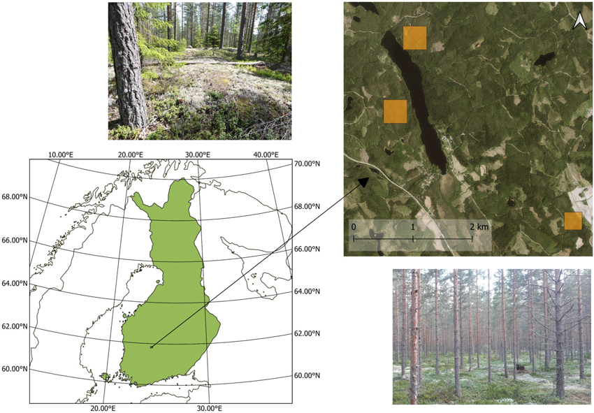
Fig. 1. Location of the study area and photos from two study stands. The in situ plots and flight plots are located within the yellow squares.
2.2 Airborne remote sensing data
Hyperspectral data were acquired on 13th July 2019 using aircraft mounted CASI-1500 and SASI-500 sensors (Hovi et al. 2022). The flight altitude was 1 km. The combined CASI and SASI data covered the spectral range 380–2450 nm and were provided in a spatial and spectral resolution of 1.25 m and 15 nm, respectively, by the Czech Globe. The data had been orthorectified to the ground surface (digital elevation model constructed from LiDAR data), and radiometrically and atmospherically corrected to yield bottom-of-atmosphere hemispherical-directional reflectance factors. The sky was partially cloudy during the data acquisition, but the flight lines used in this study were visually checked to be free of clouds and cloud shadows. The spectral bands 895–1002, 1107–1167, 1302–1527, and 1737–2050 nm were removed due to atmospheric absorption, and bands with shorter wavelengths than 450 nm and longer than 2300 nm were excluded due to reduced sensor sensitivity and increased noise, resulting in 77 spectral bands that were used in the analyses. View-zenith angles of the data used in this study varied between 0° and 10°, being on average 3.9°.
LiDAR data were collected during the same flight as the hyperspectral data using a Riegl LMS Q780 sensor. A raster digital surface model (DSM) with 0.5 m pixel size was calculated by subtracting the ground elevation from the elevation of highest laser echo in each pixel. Pixels with missing data were filled by applying a mean filter in 3×3 pixel neighborhood. A canopy height model (CHM) was then obtained by subtracting the ground elevation from the pixel values of the DSM. The CHM was later used to estimate the influence of tree canopy on the retrieved lichen cover estimates (Section 2.5).
2.3 Field measurements and data processing
2.3.1 Spectral measurements of ground cover types
Reflectance spectra of pure samples of ground cover types were measured to be used as endmembers in spectral mixture analyses. Reflectance spectra of 3–4 samples of six common lichen species (Cladonia arbuscula (Wallr.) Flot., Cladonia rangiferina (L.) F. H. Wigg., Cladonia stellaris (Opiz) Pouzar & Vězda, Cladonia uncialis (L.) F. H. Wigg., Cladonia crispata (Ach.) Flot., Cetraria islandica (L.) Ach.), three dominant dwarf shrub species (Vaccinium vitis-idaea L., Vaccinium Myrtillus L., Calluna vulgaris (L.) Hull), three common moss species (Pleurozium schreberi (Willd. ex Brid.) Mitt., Dicranum polysetum Sw., Polytrichum commune Hedw.), litter, and stone (weathered granite and granodiorite), were measured in July 2021 in overcast sky conditions, using an ASD FieldSpec4 spectrometer (350–2500 nm, spectral resolution 3 nm at 700 nm and 10 nm at 1400 and 2100 nm, serial number 18456). An average of the white reference panel measurements before and after each sample was used in the calculation of hemispherical-conical reflectance factor spectrum for each sample (Schaepman-Strub et al. 2006). We refer to these simply as reflectance spectra. The mean spectrum per cover type was used in further analyses. Measurement height varied between 15–35 cm and was adjusted for each sample so that the sample filled the entire field-of-view of the spectrometer (25˚), resulting in a circle with a radius of 3.3–7.8 cm.
2.3.2 In situ plots
Reflectance spectra of 55 plots on the forest floor with varying lichen cover and four plots without lichen (altogether 59 plots) were measured. This data set was used to test the estimation of lichen cover from in situ spectral measurements. The plots were measured during the same time and in similar conditions as the pure samples of species (Section 2.3.1). The measuring height was 1.2 m, and the corresponding radius of the sensor field-of-view on the ground was ~26.5 cm. Finally, however, the cover fractions of the ground cover types were estimated from a circle with a radius of 21.5 cm from the center of the plot, because 95% of the signal recorded by the spectrometer in the visible bands originates from that area (Hovi et al. 2020). The plots were photographed from above and the species fractions within the plots were estimated in the field. The final cover fraction estimation was done from the photographs by placing a regular grid of 90–130 points (due to varying image resolution) on the 21.5 cm radius circle, and recording the visually estimated ground cover type co-occurring each point. Example photographs of the in situ plots are presented in Fig. S1 in Supplementary file S1, and information on forest floor cover in the plots in Table 1. During the measurement, the receiver of the sensor was carefully leveled and pointed at the center of a 1 m square laid on the ground (with estimated accuracy of 5 cm).
| Table 1. Mean and range of percentage cover of ground cover types in the in situ and flight plots. | ||||
| In situ plots | Flight plots | |||
| Mean (%) | Range (%) | Mean (%) | Range (%) | |
| Lichens | 30.9 | 0–90 | 30.7 | 0–82 |
| Vascular plants | 30.7 | 0–85 | 33.9 | 0–72 |
| Vaccinium vitis-idaea | 23.5 | 0–60 | 22.2 | 0–48 |
| Vaccinium myrtillus | 0.7 | 0–39 | 2.7 | 0–27 |
| Calluna vulgaris | 6.4 | 0–48 | 8.6 | 0–52 |
| Other vascular plants | 0.2 | 0–8 | 0.4 | 0–3 |
| Mosses | 13.3 | 0–42 | 13.4 | 0–42 |
| Litter | 25 | 6–59 | 21.8 | 6–41 |
| Stone | 0 | 0 | 0.2 | 0–4 |
Spectral regions with atmospheric and instrumental noise (1330–1490 nm, 1750–2050 nm, and above 2300 nm) were removed from all measured spectra, resulting in 1488 spectral bands that were used in the analyses. The spectra were smoothed using the Savitzky-Golay filter. A second order polynomial and a window size of 15 nm for wavelengths up to 1000 nm, 39 nm for wavelengths between 1000–2050 nm, and 51 nm for wavelengths above 2050 nm were used.
2.3.3 Flight plots
Ground cover in 32 plots of 2×2 m size (see Fig. S2 in Suppl. file S1 for examples) was estimated to assess if it is possible to discriminate lichen from other ground cover types using hyperspectral airborne data. The locations of the plots were subjectively selected from small (ca. 3.5–7 m) canopy openings in which there were no trees obscuring the view of the airborne hyperspectral sensor to the plot and which ensured variability of ground cover in the data. The 2×2 m plots were accurately positioned by performing a terrestrial laser scanning (with Leica P40 Scan Station) of each plot, and co-registering the TLS data with airborne LiDAR data, using treetops as control points. Each 2×2 m plot was further divided into four 1×1 m quadrats to enable high resolution photographs of the ground cover. Species fractions in the quadrats were visually estimated in the field, and each quadrat was photographed from above. The pixel of the airborne hyperspectral data coinciding with the center of each flight plot was selected for the analysis (Section 2.4.), and the cover fractions of each ground cover type in the pixel were estimated by placing a grid of 100 points on the photograph of each 1×1 m quadrat, and estimating the cover fractions based on those grid points that fell inside the pixel of the airborne hyperspectral data. In the subsequent text, the term “flight plot” refers to the area of the 2×2 plot that coincides the pixel of airborne data.
2.4 Estimation of lichen cover from hyperspectral data using multiple endmember spectral mixture analysis
2.4.1 Background
In linear spectral mixture analysis, the reflectance spectrum of a pixel is modeled by the spectra (endmembers) of its constituent cover types (Settle and Drake 1993):
![]()
where Rs is the pixel reflectance in spectral band s, fk represents the fractional cover (abundance) of cover type k (of N) within the pixel, rk,s is reflectance of cover type k in spectral band s, and es is the residual error in spectral band s.
The forest floor composition within and across forest stands varies according to, at least, topography and microtopography, soil type, tree cover and species composition, successional stage and disturbance and management history. The spatial variation in forest floor composition can make it difficult to estimate the abundance of certain ground cover types, such as lichens, using a single endmember combination for all image pixels. This is particularly true since the similarity of spectra of different ground cover types would often inhibit the use of several endmembers in one model. One way to overcome the issue of spatial variability in endmembers is to use the multiple endmember spectral mixture analysis (MESMA) (Somers et al. 2011). In MESMA, multiple candidate models, constituting typically of two to three or four endmembers, are estimated for each pixel. The model with the smallest root mean squared error (RMSE) and typically fulfilling several criteria is then chosen for a pixel (Roberts et al. 1998).
2.4.2 Endmember selection
Altogether 130 two-to-four endmember models were estimated for each in situ plot and flight plot. For flight plots, the endmember spectra were resampled to the spectral resolution of the airborne data before the analysis. The models included all possible (non-overlapping) 2–4 combinations of the nine endmembers: average of the in situ measured reflectance spectra of 1) Cladonia arbuscula, 2) C. stellaris, 3) C. rangiferina, 4) Vaccinium vitis-idaea, 5) Calluna vulgaris, 6) Pleurozium schreberi and 7) litter, as well as average reflectance spectra of 8) C. arbuscula and C. stellaris, 9) all measured Cladonia species (Section 2.3.1.). The spectra of C. arbuscula and C. stellaris were very highly correlated and they occurred often together, which is why their mean was treated as one endmember. Note that no model included ‘overlapping’ endmembers, that is, for example, C. arbuscula and the average of all Cladonia species endmembers were never in the same model. Pleurozium schreberi was used as the only moss endmember, although small fractions of Dicranum polysetum were observed in many plots. However, the spectra of Pleurozium schreberi and Dicranum polysetum were very similar (Pearson’s correlation coefficient 0.997). Other vascular plants that occurred as minority in some plots (Vaccinium myrtillus, Empetrum nigrum, grasses, small tree seedlings) would likely be classified as Vaccinium vitis-idaea or (more rarely) Calluna vulgaris. Spectra of Cetraria islandica and Polytrichum commune were not used, as Cetraria islandica did not occur in the plots, and Polytrichum commune only rarely.
Subsets of spectral bands were selected to remove redundant spectral bands and enhance the separability between endmembers (Van der Meer and Jia 2012). We computed the covariance matrix of the scaled spectra of the most common ground cover types (endmembers) (Vaccinium vitis-idaea, Calluna vulgaris, Pleurozium schreberi, litter and Cladonia arbuscula or Cladonia rangiferina) and chose the spectral bands based on their low correlation with other bands and endmembers, determined from the covariance matrix and the values of the first eigenvector (Rees et al. 2004). This and comparison of the results using different band combinations yielded eight spectral bands: 400, 492, 670, 760, 875, 1716, 2051 and 2081 nm, that were used for the in situ plots. The correlations between endmembers in these bands were slightly lower than when using all bands, yet still high. For example, Pearson’s correlation coefficient between spectra of Cladonia arbuscula and litter, Vaccinium vitis-idaea and Pleurozium schreberi were 0.62, 0.88, 0.88 in the eight bands, and 0.70, 0.91, 0.93 in all bands. Several band combinations produced approximately as good results, and the correlations between endmembers in some band combinations were slightly smaller than in the one that was used, but the fit of the measured and estimated lichen cover was poorer. This could result from, e.g., scattering of radiation between ground cover types. In the airborne hyperspectral data, however, the selected band combination (note that band 400 nm was not usable in the airborne data due to high atmospheric scattering and low sensor sensitivity) did not yield a better agreement between estimated and measured lichen cover than using all bands. A further examination showed that excluding the shortwave infrared (SWIR) bands clearly improved the results in the flight plots (although correlations between endmembers increased). Finally, the spectral bands 496, 695, 767, 867 and 1273 nm were chosen in the airborne data. To enable a comparison to commonly used multispectral data, the data were resampled to the spectral resolution of Sentinel-2 MSI (10 and 20 m spatial resolution). The band combinations that produced the best agreement between measured and estimated lichen cover in the in situ plots (442.7, 492.4, 664.6, 782.8, 832.8, 1613.7 and 2202.4 nm) and in the flight plots (492.4, 559.8, 664.6, 704.1, 782.8 and 832.8 nm) were used.
2.4.3 Model selection
Previous studies have shown that spectral mixture analysis is sensitive to the reflectance level of the used spectra, which is usually tackled either by employing a “shade” endmember (Roberts et al. 1998; Dennison et al. 2004) or by using normalized spectra (Wu 2004; Morison et al. 2014; Kuusinen et al. 2021). We normalized the reflectance spectra of endmembers, in situ plots and flight plots by dividing the reflectance in each spectral band of a spectrum by the sum of reflectance values in that spectrum.
The best model for each in situ plot and flight plot was selected from the 130 candidate models based on the following criteria: the resulted cover type abundances must be within 0–1 and their sum 0.99–1.01. The results were categorized based on the number of explanatory variables (endmembers, 2–4), and a model from a category with one more endmember could be chosen only if the decrease of RMSE between the best model of a lower category and the best one from that category exceeded certain threshold. By comparing the estimated and measured lichen cover fractions with different thresholds, we ended up using a relative threshold, in which a model from a category with one more endmember was chosen, if the decrease in the smallest RMSE between the two categories was more than 12% of the smallest RMSE of the two-endmember category. Using this threshold, the number of endmembers in a model was four in 15% and 3%, three in 68% and 53%, and two in 17% and 44% of the models chosen for in situ and flight plots, respectively, based on the above mentioned eight and five spectral bands.
2.5 Examination of the factors affecting the results
To understand possible estimation errors of lichen cover in the plots, we calculated an “optimal” spectrum for each in situ and flight plot, i.e., a spectrum predicted based on the visually estimated cover fractions and the spectra of individual cover types or species. For this, the fractional cover of each lichen species was obtained by multiplying the field-recorded species-specific cover fractions by the total lichen cover estimated from the photographs (Sections 2.3.2. and 2.3.3.), as lichen species could not be identified reliably from the photographs. Then, we calculated the relative change from measured to “optimal” spectrum in each spectral band as: loge(measured reflectance / optimal reflectance) (Törnqvist et al. 1985). This was done to evaluate in which wavelength regions the spectra measured by the spectrometer or airborne hyperspectral sensor and the “optimal” spectra deviated the most.
Finally, we investigated how the presence of tree canopy influences the estimated lichen cover in flight plots. Tree canopy proximity was approximated by the proportion of pixels of the canopy height model (spatial resolution 0.25 m2), that had a height of at least 3 meters, of all pixels within a circle of 4 m radius from the flight plot center. Due to proximity effects, closely located trees were hypothesized to increase the differences between estimated and measured lichen cover.
3 Results
3.1 Spectral data
In situ measured mean spectra of selected species and litter are shown in Fig. 2, and these spectra are also provided in Suppl. file S2. The Cladonia species C. stellaris, C. arbuscula and C. rangiferina had a relatively high reflectance in all spectral regions, although in the near-infrared (NIR) region the reflectance was lower than that of the Vaccinium vitis-idaea. The absorption feature in the chlorophyll absorption area in the red was also less deep than in Vaccinium vitis-idaea, Calluna vulgaris and Pleurozium schreberi. The less common Cladonia crispata had a clearly lower reflectance and less steep red edge than the other Cladonia species. Reflectance spectra of flight plots with high lichen cover deviated from those with no or a little lichen, which was also demonstrated by the increasing NDVI with decreasing lichen cover (Fig. 3).
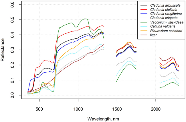
Fig 2. In situ measured reflectance spectra of selected species and litter. Data are provided in the Supplementary file S2.
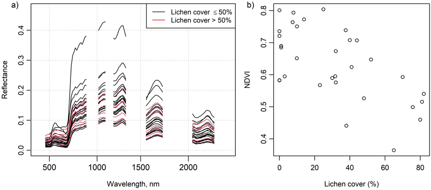
Fig. 3. Figure on the left (a) shows the airborne spectra of the 32 flight plots. Red color indicates a greater than 50% lichen cover in a plot. Figure on the right (b) shows normalized difference vegetation index (NDVI) calculated from the airborne spectra plotted against percentage lichen cover in the flight plots. NDVI was calculated using spectral bands centered at 667 nm and 838 nm.
3.2 Estimation of lichen cover
Lichen cover in the in situ plots was accurately estimated using multiple endmember spectral mixture analysis (Fig. 4). A subset of eight spectral bands produced approximately as good agreement between estimated and measured lichen cover than using all 1488 spectral bands. Lichen cover estimates derived for the flight plots, on the other hand, were less accurate than for the in situ plots (Fig. 5). The best agreement between measured and estimated lichen cover in the flight plots was obtained with a band subset that had no bands from the SWIR region (Fig. 5). When the spectral data were resampled to the spectral resolution of Sentinel-2, slightly poorer results were obtained for both in situ plots and flight plots, than when the best performing band combinations from hyperspectral airborne data were used (Fig. 6).
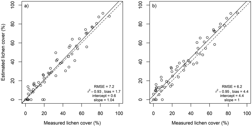
Fig. 4. Estimated versus measured lichen cover in in situ plots as well as root mean square error (RMSE), coefficient of determination (r2), intercept and slope of linear regression. Dashed lines represent 1:1 line. Results derived using a) all spectral bands (n = 1488), b) spectral bands at 400, 492, 670, 760, 875, 1716, 2051 and 2081 nm.
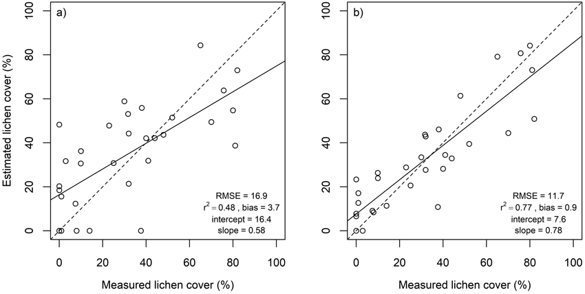
Fig. 5. Estimated versus measured lichen cover in flight plots as well as root mean square error (RMSE), coefficient of determination (r2), intercept and slope of linear regression. Dashed lines represent 1:1 line. Results derived using a) all spectral bands (n = 77), and b) spectral bands at 496, 695, 767, 867 and 1273 nm.
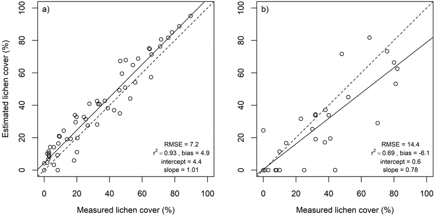
Fig. 6. Estimated versus measured lichen cover as well as root mean square error (RMSE), coefficient of determination (r2), intercept and slope of the linear regression in in situ plots (a) and in flight plots (b) when their spectra were resampled to spectral resolution of Sentinel-2. Dashed lines represent 1:1 line.
The average relative changes from measured to “optimal” spectra were largest in the SWIR region and near the chlorophyll absorption region in the red (Fig. 7). The measured reflectance in these regions was generally lower, and reflectance in NIR higher than that based on the ground cover type proportions and spectra. The differences in NIR and SWIR were larger in the flight plots than in the in situ plots. The differences imply that the measured spectra resembled on average more the spectra of green vegetation (Fig. 2) than the “optimal” spectra. In the in situ plots, the relative change in red was strongly correlated (Pearson’s correlation coefficient was –0.8) with the cover of dwarf shrubs that are generally taller than lichen, litter and moss, i.e., Vaccinium vitis-idaea, Calluna vulgaris and V. myrtillus (in one plot only) (Fig. 8). This phenomenon was not observed in the flight plots.
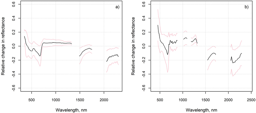
Fig. 7. Average of the relative changes from measured to “optimal” spectra, and their standard deviation, in a) in situ plots and b) flight plots.
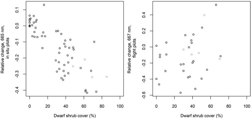
Fig. 8. Relative change from measured to “optimal” reflectance in spectral band 665 nm (in situ plots) or 667 nm (flight plots) versus measured cover of dwarf shrubs. Dwarf shrubs include Vaccinium vitis-idaea, Calluna vulgaris and Vaccinium myrtillus. Grey circles indicate plots with no lichen.
When all bands of the airborne hyperspectral data were used, low tree canopy proximity (Section 2.5.) was associated with overestimation and high tree canopy proximity with underestimation of lichen cover. The influence of nearby trees was less evident when the analysis was based on the subset of the five selected spectral bands (Fig. 9).
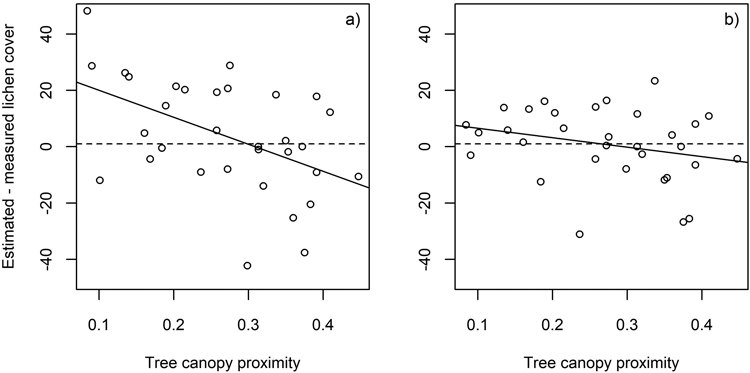
Fig. 9. The difference between estimated and measured lichen cover in the flight plots plotted against tree canopy proximity. Results derived using a) all spectral bands (n = 77) (r2 = 0.24), and b) spectral bands at 496, 695, 767, 867 and 1273 nm (r2 = 0.07).
4 Discussion
4.1 In situ versus airborne hyperspectral data in spectral mixture analysis
The estimation of lichen cover in the in situ plots was clearly more accurate than in the flight plots. This can be explained by the better match of the area from which the cover fractions of ground cover types were estimated and the area from which the signal received by the hyperspectral sensor originated from in the in situ plots compared to the flight plots. In other words, the signal recorded by the airborne hyperspectral sensor was impacted by the surrounding forest canopy as well as included residual errors due to possibly imperfect atmospheric correction and small geolocation errors, that were almost absent in the in situ measured surface reflectances. Shadow casting on forest floor during the airborne data acquisition in sunny conditions, as well as using endmembers that are measured in diffuse illumination conditions, may also complicate the interpretation of the results.
MESMA enabled the estimation of lichen cover in forests where the forest floor composition varies spatially. The average number of endmembers in models chosen for flight plots was smaller than in models chosen for in situ plots. This agrees with observations made in earlier studies: low contrast endmembers are dampened by high noise levels (Sabol et al. 1992; Drake et al. 1999), that is, the ability of mixture analysis to separate highly correlated endmembers is better using in situ measured spectra with higher signal-to-noise ratio compared to the airborne hyperspectral data. The observation that only on average two to three endmembers could be used in mixture models based on remote sensing data emphasizes the advantage of an approach in which the endmembers are let to vary on a per pixel basis.
Other observations concerning the use of multiple endmember spectral mixture analysis were that, particularly in the case of no-lichen endmembers and for airborne data, the selected endmember combination was in many cases not the “closest to real” endmember combination, even though also the “closest to real” combination would also have produced sensible cover fractions. That is, the differences in RMSEs between model candidates were sometimes very small. This leads to the second observation that increasing the number of endmembers used in the models (not the number of endmembers per model but considering more endmembers and therefore having more model candidates) did not improve the results. When too many (possibly rare) endmembers are used and the number of models increases, the possibility to obtain the smallest RMSE for a pixel by a model that is best only by chance, increases.
We estimated lichen cover in canopy openings from hyperspectral data, and to date, we are not aware of other similar studies. Thus, our results are not directly comparable to those of previous studies, but comparisons can help to gain understanding about the performance of different methods. The agreement of our measured and estimated lichen coverage in the flight plots (r2 = 0.77, RMSE = 11.7) was higher than in studies conducted in forested regions, but in the same magnitude than in studies from tundra areas, which emphasizes the difficulty in estimating lichen cover accurately in the presence of obscuring tree canopy. Silva et al. (2019) predicted lichen presence and biomass in Canadian boreal forests using information on environmental variables and spectral indices from Landsat, and found that both were best predicted by ecosite, canopy closure and time-since-fire (R2 of final biomass prediction 0.39). Likewise in Canada, Hillman and Nielsen (2020) predicted ground lichen biomass using the blue band from KOMPSAT and LiDAR derived canopy cover, which together explained 35% of the variation in measured lichen biomass. In a forest-tundra area in Alaska, Nelson et al. (2013) could explain 37% of the variation in cover of usnic lichens based on only elevation and Landsat 7 ETM+ bands 1 and 7, while variation in cover of other lichen groups was not as well explained. Kennedy et al. (2020) used machine learning to model lichen coverage across a large area in northern Canada and Alaska using Landsat TM imagery and topographical and climate data and reported an r2 value of 0.6 and RMSE of 10.4%. Falldorf et al. (2014) developed a spectral index, called Lichen Volume Estimator (LVE), which they employed in an alpine lichen heath community for lichen volume estimation from Landsat TM images, and obtained an average adjusted R2 value of 0.67 (SD = 0.115) for tenfold cross-validation.
4.2 Wavelength selection and sources of uncertainty
The subset of spectral bands selected for the unmixing analysis using the in situ hyperspectral data included three visible (400, 492 and 670 nm), two near-infrared (760 and 875 nm) and three shortwave infrared (1716, 2051 and 2081 nm) bands. Two of the visible bands (492 and 670 nm), located in the blue and red chlorophyll absorption areas, and the near-infrared bands (760 and more roughly 875 nm) agree with those used by Huemmrich et al. (2013), who studied the discrimination of functional types in a tundra site based on their in situ measured spectra in the 310–1130 nm range. Based on stepwise discriminant analysis, they ended up using wavelengths 488, 671, 712, 763 and 834 nm in estimating the coverage of vascular plants, mosses, lichens, and nongreen materials using linear spectral unmixing. We also tested the proposed wavelength combination for the in situ plots but did not achieve as good results as using the above-mentioned set of eight spectral bands. This suggests that also measuring the SWIR region when estimating ground cover type abundances from in situ measured spectra is recommendable.
Interestingly, however, the SWIR region needed to be excluded to achieve the best agreement between measured and estimated lichen cover when using airborne hyperspectral data (tested also for numerous other band combinations than those shown here). This contrasts with the results obtained for the in situ plots and could refer to the influence of tree canopy or different lichen water content during the flight and the spectral measurements of endmembers. Indeed, the lichen samples measured to be used as endmembers in 2021 were very dry, but during the acquisition of the airborne data in 2019 the lichen water content was most probably at least slightly higher (according to weather statistics). Higher lichen water content has been associated with lower reflectance in SWIR (Granlund et al. 2018), which would fit the observation that the flight plots had on average clearly lower reflectance in the SWIR than the “optimal” flight plot spectra (based on the field measured cover fractions and pure spectra) (Fig. 7). However, also the influence of green tree canopy on flight plot reflectance, through scattering of radiation by the tree crowns, would be to decrease VIS and SWIR and increase NIR reflectance; all these changes are observable in Fig. 7. and Figs. S8–S10 in Suppl. file S1. The amount of tree canopy around the flight plots was at least weakly related to the estimation errors of the lichen cover (Fig. 9), even though these canopy parts should not have been in the line of sight of the sensor to the plot. The effect of tree canopy on flight plot reflectance could also vary according to whether the plot was in sun or tree shade during the airborne data acquisition, which is unknown. However, the lower VIS and SWIR and higher NIR reflectance of the measured compared to the “optimal” spectra was visible also in most of the in situ plots (Fig. 7 and Figs. S3–S7 in Suppl. file S1). This was suspected to be a result of the scattering of radiation from taller dwarf shrubs to the lower lichens, mosses, and litter, as the relative change in red was strongly negatively correlated with the cover of dwarf shrubs (Fig. 8). However, the influence of dwarf shrubs was not observable in the airborne data, and could anyhow not explain why the SWIR region performed poorly in estimation of lichen when using airborne data (but well when using in situ measured hyperspectral data). To summarize, in the in situ plots, the differences between estimated and measured cover fractions can be caused by differences between measured endmembers and the spectra of the ground cover types present in the plot, and interactions of radiation within the plot (non-linear mixing). In the flight plots, however, these sources of uncertainty are accompanied by those related to the proximity effects of tree crowns, interfering atmosphere, and varying proportions of tree shadows on the ground.
4.3 Future perspectives of remote sensing of lichen cover
We hypothesized, that hyperspectral data would be superior to multispectral data for separation of lichens from other ground cover types. The hypothesis was supported by the fact that band selection had a large impact on the agreement between measured and estimated lichen cover. On the other hand, the lichen cover estimates derived based on the selected bands of the hyperspectral in situ (Fig. 4b) and airborne (Fig. 5b) data were only somewhat more accurate than those based on the best-performing Sentinel-2 bands (Fig. 6a and 6b) (i.e., in situ or airborne hyperspectral data resampled to the spectral resolution of Sentinel-2). This indicates that the Sentinel-2 bands are quite well suited for lichen cover estimation, and only moderate improvement for lichen cover estimation could be anticipated from the use of the new and upcoming hyperspectral satellite missions (e.g., EnMAP, PRISMA). However, because there are considerable differences in some lichen species’ spectra at wavelengths shorter than 450 nm (e.g., Fig. 2 of this study and Kuusinen et al. 2020), the availability of remote sensing data at these wavelengths would be important for separating between different lichen species. However, retrieving accurate remote sensing data from the UV-blue region is technically challenging due to large atmospheric effects and poor radiometric sensitivity of sensors.
Some findings of this study call for further investigation. Using airborne hyperspectral data, we were able to estimate the forest floor lichen cover quite well in forest openings, but studies are needed to examine lichen cover also under tree canopies. Spectral unmixing combined with forest reflectance modeling to estimate the canopy effect could be one tool for this. Furthermore, to achieve very accurate results, scattering of radiation between ground cover types, particularly from taller vegetation to lichens, should be accounted for by using nonlinear unmixing.
Availability of research materials
Spectra of the ground cover types measured in this study are available from the Supplementary file S2. Other data are available upon request from authors.
Authors’ contributions
NK designed the methodology for this study and performed the analyses. NK and AH collected the field data. AH and MR planned and coordinated airborne data collection. All authors contributed to interpreting results and writing the article.
Acknowledgements
We thank Juho Antikainen for help during the field campaign in 2021, Maaria Nordman for information on local geology, and Jan Hanuš, Tomáš Fabiánek, Lukáš Fajmon, Karel Holouš, Jussi Juola, Ville Ranta, Daniel Schraik and staff of the Hyytiälä forestry field station for collaboration during the airborne measurement campaign in 2019.
Funding
This study was supported by the Academy of Finland (DIMEBO, grant number: 323004). This study has also received funding from the European Research Council (ERC) under the European Union’s Horizon 2020 research and innovation programme (grant agreement No 771049). The text reflects only the authors’ view and the Agency is not responsible for any use that may be made of the information it contains.
References
Ahti T, Oksanen J (1990) Epigeic lichen communities of taiga and tundra regions. Vegetatio 86: 39–70. https://doi.org/10.1007/BF00045134.
Anderson JE, Plourde LC, Martin ME, Braswell BH, Smith M-L, Dubayah RO, Hofton MA, Blair JB (2008) Integrating waveform lidar with hyperspectral imagery for inventory of a northern temperate forest. Remote Sens Environ 112: 1856–1870. https://doi.org/10.1016/j.rse.2007.09.009.
Asner GP, Martin RE, Knapp DE, Tupayachi R, Anderson CB, Sinca F, Vaughn NR, Llactayo W (2017) Airborne laser-guided imaging spectroscopy to map forest trait diversity and guide conservation. Science 355: 385–389. https://doi.org/10.1126/science.aaj1987.
Asplund J, Wardle DA (2017) How lichens impact on terrestrial community and ecosystem properties. Biol Rev 92: 1720–1738. https://doi.org/10.1111/brv.12305.
Berg A, Östlund L, Moen J, Olofsson J (2008) A century of logging and forestry in a reindeer herding area in northern Sweden. Forest Ecol Manag 256: 1009–1020. https://doi.org/10.1016/j.foreco.2008.06.003.
Colpaert A, Kumpula J (2012) Detecting changes in the state of reindeer pastures in northernmost Finland, 1995–2005. Polar Record 48: 74–82. https://doi.org/10.1017/S0032247411000581.
Colpaert A, Kumpula J, Nieminen M (2003) Reindeer pasture biomass assessment using satellite remote sensing. Arctic 56: 147–158. https://10.14430/arctic610.
Cornelissen JHC, Callaghan TV, Alatalo JM, Michelsen A, Graglia E, Hartley AE, Hik DS, Hobbie SE, Press MC, Robinson CH, Henry GHR, Shaver GR, Phoenix GK, Gwynn Jones D, Jonasson S, Chapin III FS, Molau U, Neill C, Lee JA, Melillo JM, Sveinbjörsson B, Aerts R (2001) Global change and arctic ecosystems: is lichen decline a function of increases in vascular plant biomass? J Ecol 89: 984–99. https://doi.org/10.1111/j.1365-2745.2001.00625.x.
Dennison PE, Halligan KQ, Roberts DA (2004) A comparison of error metrics and constraints for multiple endmember spectral mixture analysis and spectral angle mapper. Remote Sens Environ 93: 359–367. https://doi.org/10.1016/j.rse.2004.07.013.
Drake NA, Mackin S, Settle JJ (1999) Mapping vegetation, soils, and geology in semiarid shrublands using spectral matching and mixture modeling of SWIR AVIRIS imagery. Remote Sens Environ 68: 12–25. https://doi.org/10.1016/S0034-4257(98)00097-2.
Falldorf T, Strand O, Panzacchi M, Tømmervik H (2014) Estimating lichen volume and reindeer winter pasture quality from Landsat imagery. Remote Sens Environ 140: 573–579. https://doi.org/10.1016/j.rse.2013.09.027.
Fraser RH, Lantz TC, Olthof I, Kokelj SV, Sims RA (2014) Warming-induced shrub expansion and lichen decline in the western Canadian arctic. Ecosystems 17: 1151–1168. https://doi.org/10.1007/s10021-014-9783-3.
Granlund L, Keski-Saari S, Kumpula T, Oksanen E, Keinänen M (2018) Imaging lichen water content with visible to mid-wave infrared (400–5500 nm) spectroscopy. Remote Sens Environ 216: 201–310. https://doi.org/10.1016/j.rse.2018.06.041.
He L, Chen W, Leblanc SG, Lovitt J, Arsenault A, Schmelzer I, Fraser RH, Latifovic R, Sun L, Prévost C, White HP, Pouliot D (2021) Integration of multi-scale remote sensing data for reindeer lichen fractional cover mapping in Eastern Canada. Remote Sens Environ 267, article id 112731. https://doi.org/10.1016/j.rse.2021.112731.
Hillman AC, Nielsen SE (2020) Quantification of lichen cover and biomass using field data, airborne laser scanning and high spatial resolution optical data – a case study from a Canadian boreal pine forest. Forests 11, article id 682. https://doi.org/10.3390/f11060682.
Hovi A, Forsström P, Ghielmetti G, Schaepman ME, Rautiainen M (2020) Empirical validation of photon recollision probability in single crowns of tree seedlings. ISPRS J Photogramm 169: 57–72. https://doi.org/10.1016/j.isprsjprs.2020.08.027.
Hovi A, Schraik D, Hanuš J, Homolová L, Juola J, Lang M, Lukeš P, Pisek J, Rautiainen M (2021) Assessment of a photon recollision probability based forest reflectance model in European boreal and temperate forests. Remote Sens Environ 269, article id 112804. https://doi.org/10.1016/j.rse.2021.112804.
Huemmrich KF, Gamon JA, Tweedie CE, Campbell PKE, Landis DR, Middleton EM (2013) Arctic tundra vegetation functional types based on photosynthetic physiology and optical properties. IEEE J Sel Top Appl 6: 265–275. https://doi.org/10.1109/JSTARS.2013.2253446.
Jääskeläinen K (2011) Suomen jäkälien uhanalaisuus. In: Stenroos S, Ahti T, Lohtander K, Myllys L (eds) Suomen jäkäläopas. Norrlinia 21. ISBN 978-952-10-6804-1.
Kaasalainen S, Rautiainen M (2005) Hot spot reflectance signatures of common boreal lichens. J Geophys Res 110, article id D20102. https://doi.org/10.1029/2005JD005834.
Kennedy B, Pouliot D, Manseau M, Fraser R, Duffe J, Pasher J, Chen W, Olthof I (2020) Assessment of Landsat-based terricolous macrolichen cover retrieval and change analysis over caribou ranges in northern Canada and Alaska. Remote Sens Environ 240, article id 111694. https://doi.org/10.1016/j.rse.2020.111694.
Korpela IS (2008) Mapping of understory lichens with airborne discrete-return LiDAR data. Remote Sens Environ 112: 3891–3897. https://doi.org/10.1016/j.rse.2008.06.007.
Kuusinen N, Juola J, Karki B, Stenroos S, Rautiainen M (2020) A spectral analysis of common boreal ground lichen species. Remote Sens Environ 247, article id 111955. https://doi.org/10.1016/j.rse.2020.111955.
Kuusinen N, Hovi A, Rautiainen M (2021) Contribution of woody elements to tree level reflectance in boreal forests. Silva Fenn 55, article id 10600. https://doi.org/10.14214/sf.10600.
Kuusinen N, Juola J, Karki B, Stenroos S, Rautiainen M (2022) Reflectance spectra of common boreal ground lichen species. Mendeley Data V1. https://doi.org/10.17632/k482pn3gp4.1.
Macander MJ, Palm EC, Frost GV, Herriges JD, Nelson PR, Roland C, Russell KLM, Suitor MJ, Bentzen TW, Joly K, Goetz SJ, Hebblewhite M (2020) Lichen cover mapping for caribou ranges in interior Alaska and Yukon. Environ Res Lett 15, article id 055001. https://doi.org/10.1088/1748-9326/ab6d38.
Moeslund JE, Zlinszky A, Ejrnæs R, Brunbjerg AK, Bøcher PK, Svenning J-C, Normand S (2019) Light detection and ranging explains diversity of plants, fungi, lichens, and bryophytes across multiple habitats and large geographic extent. Ecol Appl 29, article id e01907. https://doi.org/10.1002/eap.1907.
Moffat ND, Lantz TC, Fraser RH, Olthof I (2016) Recent vegetation change (1980–2013) in the tundra ecosystems of the Tuktoyaktuk Coastlands, NWT, Canada. Arct Antarct Alp Res 48: 581–597. https://doi.org/10.1657/AAAR0015-063.
Nash TH (2008) Lichen biology. Cambridge University Press, Cambridge.
Neta T, Cheng Q, Bello RL, Hu B (2010) Lichens and mosses moisture content assessment through high-spectral resolution remote sensing technology: a case study of the Hudson Bay Lowlands, Canada. Hydrol Process 2: 2617–2628. https://doi.org/10.1002/hyp.7669.
Nordberg M-L, Allard A (2002) A remote sensing methodology for monitoring lichen cover. Can J Remote Sens 28: 262–274. https://doi.org/10.5589/m02-026.
Peltoniemi JI, Kaasalainen S, Näränen J, Rautiainen M, Stenberg P, Smolander H, Smolander S, Voipio P, (2005) BRDF measurement of understory vegetation in pine forests: dwarf shrubs, lichen, and moss. Remote Sens Environ 94: 343–354. https://doi.org/10.1016/j.rse.2004.10.009.
Petzold DE, Goward SN (1988) Reflectance spectra of subarctic lichens. Remote Sens Environ 24: 481–492. https://doi.org/10.1016/0034-4257(88)90020-X.
Pykälä J (2019) Habitat loss and deterioration explain the disappearance of populations of threatened vascular plants, bryophytes and lichens in a hemiboreal landscape. Global Ecol Conserv 18, article id e00610. https://doi.org/10.1016/j.gecco.2019.e00610.
Rees WG, Tutubalina OV, Golubeva EI (2004) Reflectance spectra of subarctic lichens between 400 and 2400 nm. Remote Sens Environ 90: 281–291. https://doi.org/10.1016/j.rse.2003.12.009.
Roberts DA, Gardner M, Church MR, Ustin S, Scheer G, Green RO (1998) Mapping chaparral in the Santa Monica mountains using multiple endmember spectral mixture models. Remote Sens Environ 65: 267–279. https://doi.org/10.1016/S0034-4257(98)00037-6.
Sabol Jr DE, Abams JB, Smith MO (1992) Quantitative subpixel spectral detection of targets in multispectral images. J Geophys Res 97: 2659–2672. https://doi.org/10.1029/91JE03117.
Sandström P, Cory N, Svensson J, Hedenås H, Jougda L, Borchert N (2016) On the decline of ground lichen forests in the Swedish boreal landscape: implications for reindeer husbandry and sustainable forest management. Ambio 45: 415–429. https://doi.org/10.1007/s13280-015-0759-0.
Schaepman-Strub G, Schaepman ME, Painter TH, Dangel S, Martonchik JV (2006) Reflectance quantities in optical remote sensing – definitions and case studies. Remote Sens Environ 103: 27–42. https://doi.org/10.1016/j.rse.2006.03.002.
Schneider FD, Morsdorf F, Schmid B, Petchey OL, Hueni A, Schimel ES, Schaepman ME (2017) Mapping functional diversity from remotely sensed morphological and physiological forest traits. Nat Commun 8, article id 1441. https://doi.org/10.1038/s41467-017-01530-3.
Settle JJ, Drake NA (1993) Linear mixing and the estimation of ground cover proportions. Int J Remote Sens 14: 1159–1177. https://doi.org/10.1080/01431169308904402.
Silva JA, Nielsen SE, Lamb CT, Hague C, Boutin S (2019) Modelling lichen abundance for woodland caribou in a fire-driven boreal landscape. Forests 10, article id 962. https://doi.org/10.3390/f10110962.
Singh A, Serbin SP, McNeil BE, Kingdon CC, Townsend PA (2015) Imaging spectroscopy algorithms for mapping canopy foliar chemical and morphological traits and their uncertainties. Ecol Appl 25: 2180–2197. https://doi.org/10.1890/14-2098.1.
Skidmore AK, Coops NC, Neinavaz E, Ali A, Schaepman ME, Paganini M, Kissling WD, Vihervaara P, Darvishzadeh R, Feilhauer H, Fernandez M, Fernández N, Gorelick N, Geijzendorffer I, Heiden U, Heurich M, Hobern D, Holzwarth S, Muller-Karger FE, Van De Kerchove R, Lausch A, Leitão PJ, Lock MC, Mücher CA, O’Connor B, Rocchini D, Roeoesli C, Turner W, Kees Vis J, Wang T, Wegmann M, Wingate V (2021) Priority list of biodiversity metrics to observe from space. Nat Ecol Evol 5: 896–906. https://doi.org/10.1038/s41559-021-01451-x.
Solheim I, Engelsen O, Hosgood B, Andreoli G (2000) Measurement and modeling of the spectral and directional reflection properties of lichen and moss canopies. Remote Sens Environ 72: 78–94. https://doi.org/10.1016/S0034-4257(99)00093-0.
Somers B, Asner GP, Tits L, Coppin P (2011) Endmember variability in spectral mixture analysis: a review. Remote Sens Environ 115: 1603–1616. https://doi.org/10.1016/j.rse.2011.03.003.
Thèau J, Peddle DR, Duguay CR (2005) Mapping lichen in a caribou habitat of northern Quebec, Canada, using an enhancement-classification method and spectral mixture analysis. Remote Sens Environ 94: 232–243. https://doi.org/10.1016/j.rse.2004.10.008.
Tømmervik H, Høgda KA, Solheim I (2003) Monitoring vegetation changes in Pasvik (Norway) and Pechenga in Kola Peninsula (Russia) using multitemporal Landsat MSS/TM data. Remote Sens Environ 85: 370–388. https://doi.org/10.1016/S0034-4257(03)00014-2.
Tømmervik H, Johansen B, Tombre I, Thannheiser D, Høgda KA, Gaare E, Wielgolaski FE (2004) Vegetation changes in the Nordic mountain birch forest: the influence of grazing and climate change. Arct Antarct Alp Res 36: 323–332. https://doi.org/10.1657/1523-0430(2004)036[0323:VCITNM]2.0.CO;2.
Törnqvist L, Vartia P, Vartia YO (1985) How should relative changes be measured? Am Stat 39: 43–46. https://doi.org/10.2307/2683905.
Yang D, Morrison BD, Hanston W, McMahon A, Baskaran L, Hayes DJ, Miller CE, Serbin SP (2023) Integrating very-high-resolution UAS data and airborne imaging spectroscopy to map the fractional composition of Arctic plant functional types in Western Alaska. Remote Sens Environ 286, article id 113430. https://doi.org/10.1016/j.rse.2022.113430.
Vuorinen KEM, Oksanen L, Oksanen T, Pyykönen A, Olofsson J, Virtanen R (2017) Open tundra persist, but arctic features decline – vegetation changes in the warming Fennoscandian tundra. Glob Chang Biol 23: 3794–3807. https://doi.org/10.1111/gcb.13710.
Wu C (2004) Normalized spectral mixture analysis for monitoring urban composition using ETM+ imagery. Remote Sens Environ 93: 480–492. https://doi.org/10.1016/j.rse.2004.08.003.
Total of 53 references.
