Maria Anna Gartner  ,
Matthias Kaltenbrunner,
Manfred Gronalt
,
Matthias Kaltenbrunner,
Manfred Gronalt
Dynamic box assignment planning in log yards
Gartner M. A., Kaltenbrunner M., Gronalt M. (2024). Dynamic box assignment planning in log yards. Silva Fennica vol. 58 no. 1 article id 23032. https://doi.org/10.14214/sf.23032
Highlights
- Seasonal change of assortments calls for dynamic box assignment planning in log yards
- Multi-period planning better suited for dynamic problem, however period per period planning improves with decreasing capacity on the log yard
- Rearrangement of assortment amounts to 8–11% of total transportation distance (loaded travelled distances of transportation vehicle)
- Considering separate box allocation (storage and ejection), which results in double stage planning of box allocation, benefits most if 10% additional volume may be cut in to clear the box.
Abstract
The situation on the log yard changes seasonally and also over the years. The quantities of assortments to be stored, their number and also the type of wood can change. To respond to this, we have developed a dynamic log yard planning model for assigning roundwood to specific ejection boxes and storage areas in order to minimise the overall transport distances of the loaded transportation vehicles on the log yard, including any possible re-allocation of assortments. The study centres on the log yard of a medium-sized hardwood sawmill in Europe, with actual cutting data from a six-month period. We are comparing a multi-period binary integer program with a model that operates on a period per period basis and a solution approach that splits the problem into two subproblems and solves them sequentially. The models undergo testing with decreasing space capacities at the storage boxes on the log yard and are compared. If capacity is continuously decreasing from 100% to 80%, then period per period planning is on average 13% worse than multi-period planning. We also investigate how the solutions change when twice as many or half as many assortments are stored at the log yard. In addition, we study how much the solutions improve when logs can be removed from the storage boxes to clear them and release them for other material in the following period.
Keywords
storage assignment;
seasonality;
binary integer program;
optimisation model;
sawmill storage
-
Gartner,
University of Natural Resources and Life Sciences, Department of Economics and Social Sciences, Institute of Production and Logistics, Feistmantelstrasse 4, 1180 Vienna, Austria
 https://orcid.org/0000-0001-8547-718X
E-mail
maria.gartner@boku.ac.at
https://orcid.org/0000-0001-8547-718X
E-mail
maria.gartner@boku.ac.at
-
Kaltenbrunner,
improvem GmbH, Holzinnovationszentrum 1a, 8740 Zeltweg, Austria
https://orcid.org/0000-0002-1178-0087
E-mail
matthias.kaltenbrunner@improvem.at
-
Gronalt,
University of Natural Resources and Life Sciences, Department of Economics and Social Sciences, Institute of Production and Logistics, Feistmantelstrasse 4, 1180 Vienna, Austria
https://orcid.org/0000-0003-0944-4911
E-mail
manfred.gronalt@boku.ac.at
Received 6 July 2023 Accepted 5 December 2023 Published 15 January 2024
Views 23547
Available at https://doi.org/10.14214/sf.23032 | Download PDF

1 Introduction
At the investigated European log yard with an annual production capacity of 30 000 cubic meters, roundwood with different lengths and diameters is delivered and measured. On the sorting line, the logs are then graded based on their specifications and sorted into ejection boxes. Subsequently, they are transported to storage boxes. There they are stored until they are processed at the sawing line, where they also have to be transported. The problem of dynamic box allocation in log yards is a practical concern. Not only does the volume of the processed roundwood vary with the changing seasons, but the way in which logging has developed over the years is also apparent at the log yard. In addition, the sawing practice and the production mix of the sawmill also undergo changes over time. Therefore, it cannot be assumed that a universally applicable layout exists; rather, the allocation plan must be adapted through an iterative process. Fig. 1 illustrates how the utilisation of the ejection box and storage box can vary with diverse demand profiles at the log yard. To achieve this, a section of the examined log yard (ejection box 10, 12, 14 and 16, storage boxes for 4-metre long logs 18 and 19 in orange, and green boxes 23 and 24 for 5-metre long logs), presented in Fig. 2, has been outlined schematically.
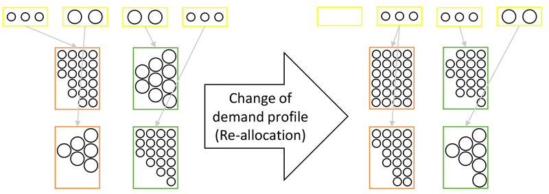
Fig. 1. Different box assignments resulting in the re-allocation of boxes in response to a schematically depicted change in demand profile (ejection boxes in yellow, storage boxes for 4-metre logs in orange and for 5-metre logs in green).
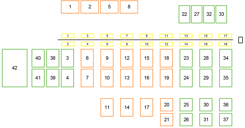
Fig. 2. Layout of the log yard with ejection boxes (yellow), along the sorting line, and storage boxes (orange and green), whereby the orange boxes have a width of 4 metres and the green boxes are suited for 5-metre long logs. To the right of the sorting line is the material feed (black).
Thereby, the previous periods’ respective layout, which refers to the allocation of logs to ejection and storage boxes, influences the allocation decisions. Thus, the effort of re-allocation at the log yard also needs to be considered. In this work, a dynamic allocation of assortments to ejection boxes along the sorting line and to storage boxes on the log yard is considered. At the log yard investigated in the paper, the material is transported with a rail mounted gantry crane, therefore no transport paths need to be taken into account. Consequently, the distance from box to box and to the material feed is calculated with the Euclidean distance and route planning is not the focus of this work. For the purpose of the paper, the log volumes of the planned periods are taken as given and no uncertainties are considered. Mathematical models are developed and tested in order to solve the dynamic allocation problem in log yards for medium-sized problems.
Several authors contribute to the topic of log yard design and logistics with different areas of investigation and propose applied solution methods. Hampton (1981) developed a log yard design procedure divided into 6 steps: collecting data of relevant activities and raw materials, modelling the material flow, working out flow relationship diagrams to identify flow priorities, determining the space needed for all activities, developing preliminary plans and evaluating these plans. The operational side of logistics is investigated by Baesler et al. (2002). The authors use a generic algorithm to minimise the production cycle in a secondary wood processing plant in Chile by optimising the number of control variables (polishing machines, sawing machines, fingerjoints machines, moulding machines and forklift cranes). By increasing the number of forklift cranes in the production line by four, the average time of the complete production cycle can be reduced by 18 percent. Inventory management in a log yard, especially in the presence of seasonality, is solved by Silver and Zufferey (2005). Tabu search and simulation are used to minimise the expected cost of lost sales when there is a known and constant demand rate but random, seasonally changing lead times. Yujie and Fang (2009) use closeness relationship values in terms of material flow to establish a good layout for a combined log yard of eight externally located forestry operations. After dividing the basic elements into operational areas, the required proximity is analysed and in turn the effective area and material flow patterns are determined. A material flow analysis at a Canadian lumber yard is studied by Beaudoin et al. (2012). The authors also investigate different loader scheduling and duty allocation strategies with a discrete event simulation. Shaik et al. (2012) apply a multi-agent-based simulation approach to increase the effectiveness of a log yard, especially its operations. In their work, they compare three different case scenarios through multi-agent based simulation with the conventional approach, employing different work order decisions for log stackers in a Swedish sawmill. In the paper by Rathke et al. (2013) an integrated approach which simultaneously takes into account log transportation time, storage capacity and yard crane deployment to reduce the log transport distance within a log yard of a medium-sized European hardwood sawmill is presented. The aim of this work is to find a better layout for the log yard by simultaneously allocating ejection and storage boxes. For this purpose, the existing layout is compared with the solutions obtained by applying an Excel-based heuristic and two optimisation models for the storage allocation to the ejection and storage boxes, both in two separate steps (double stage model, starting with the storage boxes) and simultaneously (partition model). Unlike existing work in this area, Rathke et al. (2013) use mathematical optimisation models to generate the solution. Rahman et al. (2014) implement a discrete event simulation to improve a Swedish log yard and its processes. In this approach, storage bins are effectively rearranged to minimise log stacking time. Furthermore, storage assignment with seasonal data is examined. To this end, two different planning samples, a one-month and a three-month planning sample covering a whole year, are used and compared with the existing layout. Based on the work by Hampton (1981), Robichaud et al. (2014) investigate the design and evaluate the performance of a log yard in Quebec using discrete event simulation. The authors model the material flow and develop flow priorities, evaluating the intermediate plans using the simulation model. For a layout, equipment combinations are tested for high and low utilisation and arrival rates and measured against the scheduled time utilisation and total travel distance. Huka and Gronalt (2018) give a good overview of the different logistical problems that can occur in a log yard. The authors also highlight the unsolved areas, including the dynamic box assignment problem in log yards. Furthermore, four case studies and different solution approaches are shown. Trzcianowska et al. (2019a) examined current log yard practices in the province of Quebec. The results suggest a competitive advantage through improved log yard practices, optimisation of log yard shape and layout, better coordination between forest and mill operations, and through improved ground cover. An interesting finding is that all log yards studied are affected by seasonality. The inventory variation ranges from 18 to 76 percent. The authors report, that log yards surveyed are dealing with the change in timber volume in different ways. Some report an increase in storage space with a higher inventory and an increase in machinery and labour. One log yard reports closing during the low season. Log yard efficiency is studied by Trzcianowska et al. (2019b) using data envelopment analysis. 38 log yards in Quebec are analysed in terms of efficiency, the relationship between efficiency and operational conditions, and management strategies. Technical efficiency is evaluated in terms of a complexity factor that is influenced by seasonality, size and shape of the log yard and the number and type of assortments to be handled. An automated log yard with automated storage components is studied by Pernkopf and Gronalt (2020). The authors use a discrete event simulation model to evaluate the alignment of different numbers and lengths of these automated storage components. By using two different lengths of the components, the minimum cost can be achieved for each of the 12 scenarios investigated, with 6768 eligible combinations of automated storage components evaluated. In the most recent publication, Trzcianowska et al. (2021) presents an approach for planning of log yards considering seasonality by means of discrete event simulation. In a first step, three periods of log supply are distinguished: the accumulation season, the inventory run down season, and the equilibrium season. To account for the different seasons, three designs (1, 2, and 3 loader) are tested using simulation. The authors distinguish between three performance criteria, truck cycle time, distance travelled, and equipment utilisation rate.
Although some of the papers presented investigate seasonal aspects of the log yard by simulation, we are not aware of a paper that investigates the optimised changing layout at different storage levels or product mix. To achieve this, the model of Rathke et al. (2013) is further developed. In this context, the concept of re-marshaling, which is well known in the field of container terminals, is very interesting. There, insufficient information regarding initial stacking can result in the need to reschedule retrieval operations. This occurs when containers are stacked in an order that is not reflective of the actual retrieval sequence. Automated stacking cranes are capable of rescheduling operations to move unproductive movements during retrieval operations to periods when the cranes are not engaged. This is called re-marshaling. There are commonalities in terms of handling and movement of the individual containers or logs. For this purpose, the objective function of the model by Rathke et al. (2013) is extended by a re-marshaling component and thus the optimal storage allocation is ensured at any time, taking into account the restructuring effort. This re-marshaling component corresponds to the costs of re-allocation and the time needed to reallocate assortments into different storage boxes. Kim and Bae (1998) present a method to transform an existing bay layout into a desired layout with as few container movements as possible. They divide the problem into three parts, the calculation of the desired layout, the movement planning and the task sequencing, and solve each part with a mathematical model. The re-marshaling problem with a limited time horizon is studied by Yu and Qi (2013). With the aim of minimising the waiting time of trucks picking up containers at the port, two correlated approaches are used; the calculation of optimal block space allocation for container storage and nightly re-marshaling to reorganise block space allocation. The re-marshaling is solved with a heuristic, and a simulation model validates the solution procedures. Yi et al. (2018) investigate how the repeated manipulation of containers can be reduced when estimated truck arrival times are available. Algorithms for planning pre-marshaling operations and determining storage locations for re-handled containers are presented and compared using simulation studies.
This paper enhances the existing work cited above in that it takes a dynamic approach to log yard occupancy planning. The mathematical models presented here are based on the work of Rathke et al. (2013) and are extended by a re-marshalling component and constraints for multi-periodicity. This allows the costs arising from restructuring to be included in multi-period planning; costs equivalents can be distances travelled, quantities moved or time required. In this way, optimal occupancy of the log yard is ensured at all times in the event of seasonal order situations or changing log distribution.
2 Material and methods
For this work, we expand on the established model of Rathke et al. (2013) to include periods, the possible transport of logs between the storage boxes, and all other necessary logical constraints to adapt it to multi-periodicity. As discussed in the literature review, the objective function is extended by a re-marshaling component that takes into account the distances travelled at the log yard for reassigning storage areas. The entire volume of the previous period is reassigned, either into the same storage box or into a new storage box, taking into account the distances between the individual storage boxes and the needed number of trips for the reassigned volume. Thereby, all loaded transport distances are minimised, from the ejection box to the storage box, any possible distances between reassigned storage boxes with residual material over several periods, and finally to the material feed of the sawing line.
Fig. 2 shows the layout of the investigated log yard. Along the sorting line there are 18 ejection boxes (yellow) from which a gantry crane transports the supplied assortments into 42 existing storage boxes. 23 of these storage boxes are suitable for storing 5-metre long logs (green) and 19 of the boxes are 4 metres wide (orange). The total storage capacity is divided into 40% 4-metre boxes and 60% 5-metre boxes. The crane subsequently transports the required volume from the storage boxes to the material feed. It should be noted, however, that the shorter assortments can also be stored in the 5-metre boxes, but not the other way round. On the log yard, 15 assortments are manipulated in a planning period of half a year, divided into 13 periods of two weeks. Of these, eight are 5-metre long and the diameters vary from 16 to 41 centimetres. Fig. 3 shows the total delivered, stored and consumed volume per period. Of course, the stored volume is always greater than or equal to the consumed volume. The quantities used are based on the cutting optimisation by Huka and Gronalt (2017). The estimated distances are measured on an existing log yard. The exact distribution of the individual quantities from Fig. 3 can be taken from Fig. 4. Here the respective distribution of 4- and 5-metre lengths can be }seen. Only a quarter of the total amount delivered, stored and consumed on average in the planning period is of 4 metre length. For the following two mathematical models several indices, parameter and decision variables are needed.
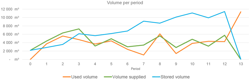
Fig. 3. Changes in inventory at the investigated log yard per planning period for half a year, total supplied volume per planning period (green), total stored volume per planning period (blue) and total used volume per planning period (orange).
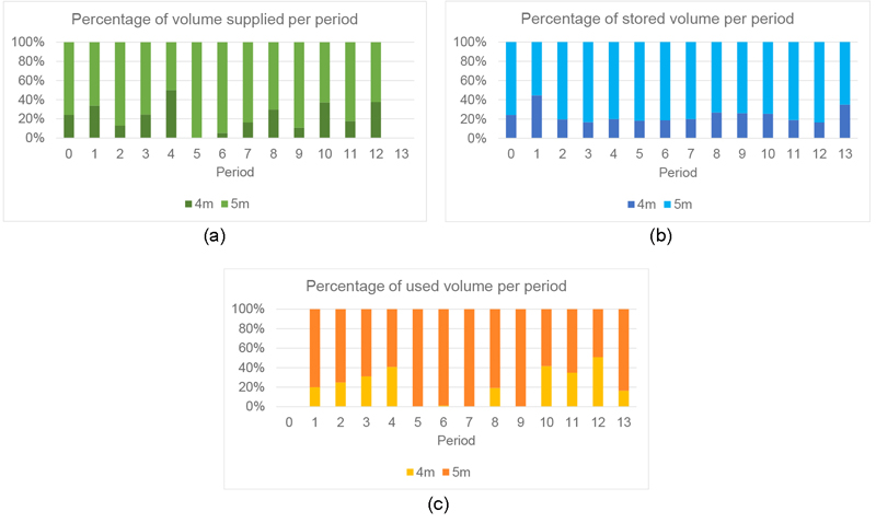
Fig. 4. Percentage distribution of the total volumes of 4- and 5-metre assortments of supplied material (a), stored material (b) and used material (c) per planning period at the log yard.
Indices:
A Set of assortments a
E Set of ejection boxes e
S Set of storage boxes s
T Set of periods t
Parameters:
Cs Capacity of storage box s
Vat Supplied volume of assortment a in period t
Na Number of trips per unit volume per assortment a, depending on the diameter of the assortment, its length and capacity of the transportation vehicle (independent of the period)
Ds Distance from storage box s to the material feed
Des Distance from ejection box e to storage box s
Dss′ Distance from storage box s to storage box s′
Uat Used volume of assortment a in period t
Bs Length of storage box s, 1 if box is of 5-metre length, 0otherwise
La Length of assortment a, 1 if assortment is 5-metre long, 0otherwise
P Percentage of the maximum additional volume that may be transported to material feed per period, in addition to the volume required for cutting in that period
Variables:
yaet 1 if assortment a is assigned to ejection box e in period t, 0otherwise
wast 1 if assortment a is assigned to storage box s in period t, 0otherwise
vaest New volume of assortment a in ejection box e and storage box s in period t
fast New volume a in storage box s in period t
qast Volume of assortment a in storage box s in period t
uast Used volume of assortment a from storage box s in period t
mass′t Volume of assortment a transported from storage box s to storage box s′ in period t
dat Additional volume of assortment a transported in period t
Table 1 shows the minimum, maximum and average value of the number of trips per assortment and the different distances between ejection box, storage box and material feed. The values for the parameter Na are averages over both lengths of assortments, but as expected, 4 metre long assortments require on average 2.6 fewer trips than longer assortments.
| Table 1. Minimum, maximum and average of the parameter values for the number of trips and distances in metres. | |||
| Parameter | Min | Max | Average |
| Na | 7.71 | 12.53 | 9.69 |
| Ds | 45.70 | 250.38 | 149.60 |
| Des | 4.38 | 200.58 | 76.85 |
| Dss′ | 1.50 | 200.03 | 76.65 |
The total available capacity of the investigated log yard is 28 506 cubic metres, divided into 40 and 60% for 4 and 5-metre storage boxes respectively.
2.1 Optimisation model
The dynamic box assignment problem is formulated below as a binary integer model. The following notation is used to specify the mathematical model:
![]()
![]()
![]()
![]()
![]()
![]()
![]()
![]()
![]()
![]()
![]()
![]()
![]()
![]()
![]()
![]()
![]()
![]()
![]()
Objective function Eg. 1 minimises the total transportation distance. On the one hand, this is the volume transported between the ejection box and the storage box; on the other hand, it is the quantity delivered to the material feed and possible reassignment quantities multiplied by the distance and the number of trips required, depending on the volume, length and capacity of the means of transport. The first constraints Eq. 2 ensure that the entire supplied volume of assortment a in period t is stored somewhere on the log yard. Constraints Eq. 3 compute the volume for each assortment a stored in box s in period t. This is the amount transported from storage box s to storage box s′ remaining from the previous period, plus the volume supplied to the log yard, minus the quantity consumed during this period. The following constraints Eq. 4 state that, in every period t, for each assortment a and storage box s, the remaining volume from the previous period must either be reassigned to another storage box or kept in the same one to ensure that no volume is lost. In addition, the next constraints Eq. 5 guarantee the correct allocation of the quantity of assortment a in storage box s′ in period t for the subsequent period. The upper limit on the right-hand side of the constraints ensures that the volume transferred to the storage box, upon assignment of the assortment, does not surpass the total of the largest amounts delivered and consumed. The same upper bound is also employed in constraint Eqs. 14–17. The following two restrictions Eq. 6 and Eq. 7 provide that storage capacity is not surpassed. The capacity of each storage box s in each period t is limited by the constraints Eq. 6. Furthermore, constraints Eq. 7 ensure that 5-metre assortments are only assigned to 5-metre storage boxes and, in contrast, 4-metre assortments, which can also be stored in larger storage boxes for 5-metre logs. Constraints Eq. 8 state that the entire required volume of an assortment a in period t is sourced from the possible storage boxes s. Additionally, more volume can removed from the box to free it up for the next period. Constraints Eq. 9 restrict the total amount of extra volume per period. The volume of assortment a that can be transported to the material feed in period t is limited by the quantity of material available in storage box s, as outlined in constraints Eq. 10. The subsequent two constraints Eq. 11 and Eq. 12 ensure the accurate assignment of each assortment a to an ejection box e per period t. The constraints Eq. 11 limit the assignment for each ejection box to a maximum of one per period, while the constraints Eq. 12 assign each assortment to exactly one ejection box per period if new volume is added during that period. Constraints Eq. 13 enforce that each storage box s per period t may only be used for one assortment at a time. The following four constraints Eqs. 14–17 establish a connection between the volume of assortment stored and consumed and the chosen assignment. These constraints govern the filling of all assortments a in storage boxes s and ejection boxes e in period t. Filling and the volume used must not exceed the maximum assortment volume per period if the assortment is assigned to the corresponding box. Restrictions Eq. 18 and Eq. 19 define the binary variables. Since the issue of allocating ejection and storage boxes simultaneously proves challenging to solve, the double stage model is introduced in the following section.
2.2 Double stage model
Based on the double stage model presented in the paper Rathke et al. (2013), where storage boxes are assigned first, and ejection boxes are chosen in a second subsequent step, the model is extended to multiple periods for dynamic assignment. This approach was chosen because the problem is easier to solve when it is split into two subproblems. In addition, the computation time is less with the double stage model.
2.2.1 Stage one
As with 315 the model described above, the allocation to storage boxes is made in stage one of the double stage model. The difference to the optimisation model Eq. 1 with constraints Eqs. 2–19 is that in step one, no ejection boxes are considered. The objective function Eq. 20 consists of the last two parts of the objective function of the overall optimisation problem Eq. 1. The distance travelled from the storage box to the material feed as well as any re-allocation distances are minimised. For the assignment, volume and capacities are taken into account. In addition, the volume from the previous period is reassigned if necessary, see constraints Eqs. 22–24, and the lengths of the assortments and boxes are considered, see constraints Eq. 26.
![]()
![]()
![]()
![]()
![]()
![]()
![]()
![]()
![]()
![]()
![]()
![]()
![]()
![]()
![]()
2.2.2 Stage two
The objective of the second stage of the double stage model Eq. 35 is to minimise the distance between the ejection box and the storage box. As in the optimisation model, the constraints Eqs. 36–40 ensure that assortments are uniquely assigned to ejection boxes and that no volume is lost between ejection box and storage box.
![]()
![]()
![]()
![]()
![]()
![]()
2.3 Period per period model
In the period per period approach, the optimisation model Eq. 1 described above is solved for each period separately under the constraints Eqs. 2–19. The new model differs only in the indices of the decision variables. These are not dependent on the period here. For the correct transfer of the stored quantities in the respective storage boxes after each optimisation, this value is saved and transferred as the initial situation in the next period. These quantities can be re-allocated into new storage boxes as needed. Now that the models used have been described, we test and validate them with a detailed numerical study.
3 Numerical experiments and results
At the investigated log yard, the raw material is divided into 15 assortments. These are sorted according to log length and diameter along the sorting line into 18 ejection boxes and then stored in 42 storage boxes until processing in the sawmill. As mentioned above, there are seven assortments with a length of 4 metres and eight assortments with a length of 5 metres. For storage, there are 19 storage boxes with a width of 4 metres, which corresponds to 40% of the total capacity at the log yard. Over the planning period under consideration, the stored quantity is distributed on average between 24% of the 4-metre assortments and 76% of the 5-metre assortments. The planning horizon is half a year with a period length of 2 weeks.
The data used and especially the volumes for used logs correspond to the data and optimisation result from the study by Huka and Gronalt (2017). Here, the objective is to maximise the contribution margin of a sawmill (net revenue minus production costs, purchasing costs for roundwood, inventory costs for raw material and products, and backorder costs for products where demand is not met in time) with available roundwood, a fixed demand and numerous cutting patterns. Since no uncertainties are considered in this paper, the stored roundwood volume per period is known in advance, as delivery and consumption are known. However, these data are based on optimisation results of the cutting planning and historical and real roundwood delivery data. Note that the computations are conducted on an Intel Core i7-5820K computer with 64GB RAM using FICO Xpress for the optimisation. Nevertheless, the standard settings of Xpress 8.6 have been tuned for the multi-period optimisation (Heursearchrootcutfreq = 2, Heursearchrootselect = 3, Cutfactor = 5) and double stage model (Heursearcheffort = 0.5, Symmetry = 0, Heursearchrootselect = 3). We have agreed to accept solutions with a maximum of 6% deviation from lower bound and best solution due to computation time. For the period per period model, however, the default settings were not changed and a gap of 0% is used, since the computing times are negligible.
In a first step, the multi-period optimisation model presented above is compared with the double stage model, see Table 2. In addition, the problem is solved with period per period planning and compared with the two other solutions. In the initial situation, there is 2.5 times as much storage volume as the maximum required per period. Starting from this given actual situation, the existing capacity is iteratively reduced by 10%. On the one hand, this can simulate a higher filling level, e.g. after wind throw, or a higher stock build-up in the log yard. On the other hand, this capacity reduction can be attributed to a lower stacking height at the log yard.
| Table 2. Comparison of transportation distances between the dynamic log yard box assignment problem multi-period optimisation model solution and those derived from the double stage model and period per period optimisation, while also considering capacity variations at the log yard. | |||||
| Available capacity | Multi-period | Double stage | Period per period | ||
| metre | metre | % | metre | % | |
| 100% | 53 203 087 | 57 105 387 | 7 | 61 048 908 | 15 |
| 90% | 54 306 150 | 59 368 512 | 9 | 61 867 595 | 14 |
| 80% | 55 315 550 | 62 079 198 | 12 | 61 195 460 | 11 |
| 70% | - | 62 887 167 | - | 63 412 692 | - |
| 60% | infeasible | ||||
If the capacity is reduced to 40% of the original capacity or even lower, which corresponds to a ratio of capacity to total volume, at the highest volume per period, of 0.998, clearly no solution can be found. Although with a reduced capacity of 50% the ratio is 1.25 and the total volume per period is always smaller than the available capacity, no solution can be found in this case either. The reason for this is that the volume of the 5-metre assortments exceeds the capacity of the 5-metre storage boxes. This would not be the case if the capacity of the 4-metre storage boxes is too small, as these assortments can also be stored in the larger boxes. If the capacity of the storage boxes is reduced to 60%, the ratio of available to maximum required storage space is 1.50. Theoretically, the storage space available for the 5-metre-long assortments is also sufficient, the ratio being 1.07 times that required. However, no solution can be found for this situation. If the available storage space is increased by 10% each, the factor increases by 0.25 each time.
Table 2 shows that the double stage model generates 7% to 12% higher transport distances than the multi-period optimisation model, depending on the available storage capacity. As expected, period per period planning is the worst suited to the problem with sufficient capacity. However, the less capacity there is in the storage boxes at the log yard, the better the results. The solutions are 15% to 11% worse than the optimal solution. Compared to the double stage solution, where the transport distances from ejection box to storage box are 100% higher on average than the multi-period optimal solution and increase with decreasing capacity, these distances are 15% lower on average in the period per period solution. Table 4 provides detailed information on this matter. As capacity becomes scarcer, the transportation distances to the material feed increase by an average of 17% when calculated with the period per period model. Nonetheless, these distances progressively decrease from 22% to 10% as storage capacity is diminished. However, when the log yard operates at 70% capacity, the period per period model incurs re-allocation distances that are 50% higher in comparison to the optimum of the multi-period model at the same capacity. The values for each objective function component are provided as supplementary information, since Table 2 only presents the overall values for the objective function across all models. The detailed breakdown of individual components is presented below. For the multi-period planning model, no integer solution could be found after 14 days of computing in the case of 70% of available storage capacity. It takes the double stage model a little over 2 days to reach a solution in this case, see Table 3. The other solutions can be found within a maximum of 7 hours. The computing times of the individual runs can be taken from the Table 3.
| Table 3. Computation time, in seconds, for multi-period, double stage and period per period planning for the dynamic box assignment problem with reduced available capacity at the log yard. | |||
| Available capacity | Multi-period | Double stage | Period per period |
| sec | sec | sec | |
| 100% | 5662 | 105 | 26 |
| 90% | 2828 | 5199 | 22 |
| 80% | 2086 | 27 713 | 41 |
| 70% | - | 195 994 | 35 |
Table 4 shows the distribution of distances among the individual factors of the objective function. Since the variance for the different capacities is not very large (maximum 3% for multi-period planning, 4% for the double stage model and 3% for period per period planning), the average values are shown.
| Table 4. Average distribution of distances over the three parts of the objective function, transport distances of delivered material from ejection box to storage box, transport distances of used material to the feeder and reallocation distances, over available storage box capacities 100% to 70% and 60% respectively. | |||
| Objective function | Multi-period | Double stage | Period per period |
| Ejection box to storage box | 12% | 22% | 9% |
| Material feed | 78% | 71% | 80% |
| Re-allocation | 10% | 8% | 11% |
With the double stage planning results, it is easy to see that in the first step the distances from ejection box to the storage boxes are not taken into account, therefore they are almost twice as high compared to the multi-period optimisation. However, in comparison, lower distances of transportation to the material feed can be achieved in the first planning step. The period per period planning generates lower distances of transport from ejection box to storage box, but higher distances to the material feed. However, the re-allocation distances are not much higher than with the two multi-period planning approaches.
The study also considers the number of delivered and consumed assortments per period, i.e. the number of assortments in stock. The current state involves a minimum of three and a maximum of nine different assortments being delivered per period. In a planning period of two weeks, a minimum of two and a maximum of eight different assortments are consumed. It is investigated how the solution changes if the assortments are divided into twice as many or half as many assortments per period. This can be explained on the one hand by a refined sorting logic and on the other hand by an extension of the assortments or an additional type of wood. In Table 5 the influence of the number of assortments on the solution of the assignment planning on the log yard can be seen.
| Table 5. Comparison of the covered distance solution of the dynamic box assignment planning in log yards of the multi-period optimisation model with the double stage model and period per period planning, in which the volume per period remains constant but the number of assortments per period is either doubled or halved. | ||||||
| # Assortments | Multi-period | Double stage | Period per period | |||
| metre | % | metre | % | metre | % | |
| ×2 | 60 560 513 | 14 | 66 256 867 | 16 | 65 868 598 | 8 |
| ×1 | 53 203 087 | 0 | 57 105 387 | 0 | 61 048 908 | 0 |
| ×1/2 | 48 407 990 | –9 | 51 362 746 | –10 | 55 840 717 | –9 |
Table 5 shows the alteration of the solution with a changed number of assortments compared to the respective solution of the initial situation. Doubling the number of assortments has the least impact on period per period planning. In this situation, the period per period planning even achieves a better solution than the double stage model, even though the re-allocation distances in particular increase by almost 40%. For the two multi-period solutions, the transport distances increase by about 15% to 60 560 513 metre and 66 156 867 metre respectively. This is due to the fact that the distances from the ejection box to the storage box and from there to the material feed have increased. Rearrangement distances even decrease with both solution approaches. Dividing the number of assortments in half leads to approximately 9% less transport distances for all three solution methods. In this case, the transport distance to the material feed and any re-allocation distances decrease with all three models. For the multi-period and period per period optimisation model, however, the transport distances between the ejection box and storage box increase. The allocation to the three factors of the objective function is relatively unchanged with different numbers of assortments, and deviates from the average values from Table 4 by a maximum of 3% for all models examined. In the following analysis shown in Table 6, a storage box can be cleared in spite of the required cutting volume because it is allowed to deliver up to 10% more volume per assortment and period to the material feeder. In the models studied, the excess quantity is not deducted from the quantity demanded in the next period; such additional quantity can be considered as a production buffer. This method of emptying a box aims to prevent needless re-allocation of small residual quantities in order to obtain a well-placed, previously occupied box.
| Table 6. Percentage change in results of covered distance for the dynamic box assignment problem in log yards if 10% volume is allowed to be taken from the storage boxes in addition to the demanded quantity used at the saw. | ||||||
| Available capacity | Multi-period | Double stage | Period per period | |||
| metre | % | metre | % | metre | % | |
| 100% | 53 132 715 | –0.13 | 56 432 380 | –1.18 | 60 986 796 | –0.10 |
| 90% | 54 127 494 | –0.33 | 58 741 336 | –1.06 | 61 811 628 | –0.09 |
| 80% | 55 174 836 | –0.25 | 60 271 310 | –2.91 | - | - |
| 70% | 56 614 306 | - | 62 514 704 | –0.59 | - | - |
The additional material removal to clear a box has only a small impact on the transport distances, see Table 6. Here, we compare the solution without the additional allowed amount and different capacity levels with the solution obtained when up to an additional 10% volume may be removed. The transport distances are reduced by a maximum of not quite 3% by this measure. The distribution of the individual factors of the objective function is the same for the multi-period model with additional 10% as shown in Table 4. The two other models deviate from the values shown above by a maximum of 1%. It should be mentioned that over the planning horizon of 13 weeks, a total of between 42 and 49 solid cubic metres are additionally consumed, depending on the available storage capacity. The maximum volume per period and assortment is four solid cubic metres. In total, a maximum of 10 solid cubic metres more are consumed per period, with 200 solid cubic metres being sawn per half hour. Furthermore, it is ensured that sufficient raw material is available to supply the saw in the further course of planning. However, since period per period planning does not guarantee this by not planning for the future and focusing on one single period at a time, it is not suitable for this analysis. When the storage capacity is reduced to 80%, additional material is supplied to the material feed, which is lacking in the following period. Thus, one-period planning cannot be solved in this case.
4 Discussion
Many log yards do not have a standard layout. These have naturally grown with time and their requirements. This often leads, at least in Europe, to non-contiguous storage areas or reserve areas for lesser rotated logs. Some log yards are located along a river or public road, others are part of a larger wood processing company and share storage space with other products. It is precisely in such environments that dynamic box assignment planning in log yards can lead to considerable savings. Multi-period planning can save more than 13% compared to planning per period, which in itself is an improvement over the status quo. When using the dynamic box assignment planning models in log yards, it is known at any time, where which diameters and lengths are stored. These data is supported by GPS guided log yard logistics, which is another advantage of the application. In this paper, we have assumed known stock quantities and cutting volumes. For the actual application in the sawmill, one can assume the contracted log purchase volumes on the one hand and the sawn timber delivery liabilities (and the log volumes defined for this by default by the cutting patterns used) on the other hand. The quantities and general composition of roundwood in a log yard change not only seasonally, but also over time. In addition, the model can be fed continuously with the updated data at the roundwood yard. This information is to be taken out of an ERP (Enterprise Resource Planning) system in use. Close cooperation between purchasing, yard management and the sales department also makes it possible to estimate the required quantities of delivered and consumed roundwood even better, which leads to a better result at the log yard. Due to cutting rates, the storage allocation must also adapt so that the layout remains optimal. In this way, the required overall transport distances can be kept to a minimum and unnecessary kilometres, resulting in fuel or energy consumption and consequently spent time, can be avoided. The costs for the means of transport used can either be evaluated with the current electricity or fuel costs, or only with the distance travelled. Thus, we have developed an exact model to solve the dynamic box assignment problem in log yards. This builds on the work of Rathke et al. (2013), which was extended by periods and a re-marshalling factor. To tackle the dynamic box assignment problem in log yards, we compare a multi-period model with a double stage approach and a period per period model. In the double stage approach, the problem is divided into distinct subproblems. First, the allocation of assortments to storage boxes and in a second step, the allocation of ejection boxes to storage boxes is solved. Not surprisingly, the multi-period model gives superior outcomes. However, when dealing with storage boxes with less capacity, it is unable to find a solution within a reasonable computational time. If the available capacity at the log yard is reduced by 30%, no solution will be found in the given calculation time. In comparison, the double stage model deteriorates from 7% to 12% when the log yard capacity decreases from 100% to 80%. The computation time, however, extends from roughly 2 minutes to over 2 days. The period per period model, on the other hand, improves as capacity decreases, resulting in 15% to 11% worse results than the multi-period model. At first, this seems surprising, but closer examination of the results provides an explanation. In contrast to the multi-period planning, where the transport distances to the material feed increase with less available capacity, in the period per period model the distances decrease. This part of the objective function accounts for approximately 78% and 80% of the total distances. Thus, the improvement in the performance of the period per period model compared to the multi-period model is evident. The calculation time for each instance takes a few seconds. However, on average, it is 13% worse than multi-period planning. At 70% available capacity, period per period planning is 0.84% worse than the double stage model. In multi-period and period per period planning, the individual factors are distributed approximately equally. 10% are re-allocation distances, about 80% are transport movements between storage box and material feed and the remaining 10% of the objective function are transport distances from the ejection box to the storage box. If we divide the problem into two parts and first minimise the distances between the storage box and the material feed, the result are lowertransport distances of about 70%. The re-allocation distances are similar to the other two models, at around 8%. For the case where only half as many assortments are stored on the log yard, all models perform about 9 to 10% better than in the original test configuration. However, when there are twice as many assortments, the period per period planning is outperformed by the multi-period and double stage models, which achieve 14% and 16% better results, respectively. When 10% more volume is allowed to be removed from a storage box than is required to clear a box, results improve for all models studied. The highest improvement of about 2.9% is obtained at 80% of capacity with the double stage model. For this situation, however, no solution can be found with the period per period model, since it plans too myopic. In general, it would make sense to use the dynamic box assignment planning model in log yards at least every quarter or when there is a major change in procurement quantities. Through regular application, the log transport costs can be saved on a continuous basis. The storage capacities available at the log yard must be determined precisely in advance. In order to accurately model the conditions, all distances have to be measured, the dimensions of the storage boxes have to be determined, and the maximum stacking height has to be set. Furthermore, the maximum quantity that a transport gripper can load must be determined, and thus the required number of trips per assortment calculated. In addition, the management of the log yard must agree upon a practical and feasible handling of the storage principle (last in first out, first in first out). As the model presented is based in crane movements, the same models can be used for log yards with stackers. To reflect reality, distances must be measured against the routes and reconciled with the log yard management.
5 Conclusion and further work
The models presented here have been sufficiently tested for their applicability. In a next step, the models are to be calculated using different or expanded data sets. As a result, not only do the number, quantity and distribution of assortments change, but also the overall layout of the log yard. The storage areas do not have to be contiguous, and several material feeds can exist. The chosen means of transport in the log yard is also irrelevant for the mathematical model. The distances between the individual boxes (ejection and storage box) and the material supply must be known. The distances can be calculated along the existing routes or Euclidean. In addition, stronger seasonal amplitudes and assortment changes are analysed in a further step. Another extension of the existing model is to investigate how to deal with the additional amount of logs that can be taken out of a storage box to empty it for cutting. In this paper, it is assumed that this will not lead to a reduction in the amount of cutting required in the future, but will serve as a production buffer. Moreover, the presented models can be adapted for other log yards in the wood-based panel industry. Here, it is only necessary to differentiate between the various stored assortments and their requirements for the storage area. In a next step, we will develop problem specific matheuristics and compare them with the optimal solutions found. Thus, we hope to find relatively good solutions in relatively short computation time.
Declaration of openness of research materials, data, and code
Data and code available on request from the corresponding author.
Author’s contribution
M.A.G. participated to the data acquisition and drafted the manuscript. M.A.G. and M.K. carried out all numerical analyses. All authors participated to defining research questions and design of the work, the numerical analysis, interpretation of data and results, revising the manuscript and approved the final version to be published. M.G. defined research outline and activities supervised the whole project.
Funding
Open access funding provided by University of Natural Resources and Life Sciences Vienna (BOKU).
References
Baesler FF, Moraga M, Ramis FJ (2002) Productivity improvement in the wood industry using simulation and artificial intelligence. In: Proceedings of the Winter Simulation Conference, San Diego, CA, USA, pp 1095–1098. https://doi.org/10.1109/wsc.2002.1166362.
Beaudoin D, LeBel L, Soussi MA (2012) Discrete event simulation to improve log yard operations. INFOR 50: 175–185. https://doi.org/10.3138/infor.50.4.175.
Hampton CM (1981) Dry land log handling and sorting: planning, construction, and operation of log yards. M. Freeman Publications.
Huka MA, Gronalt M (2017) Model development and comparison of different heuristics for production planning in large volume softwood sawmills. Eng Optim 49: 1829–1847. https://doi.org/10.1080/0305215X.2016.1271882.
Huka MA, Gronalt M (2018) Log yard logistics. Silva Fenn 52, article id 7760. https://doi.org/10.14214/sf.7760.
Kim KH, Bae JW (1998) Re-marshaling export containers in port container terminals. Comput Ind Eng 35: 655–658. https://doi.org/10.1016/S0360-8352(98)00182-X.
Pernkopf M, Gronalt M (2020) A simulation-based sizing approach for automated log yards. Simul Modell Pract Theory 104, article id 102123. https://doi.org/10.1016/j.simpat.2020.102123.
Rahman A, Yella S, Dougherty M (2014) Simulation model using meta heuristic algorithms for achieving optimal arrangement of storage bins in a sawmill yard. J Intell Learn Syst and Appl 6: 125–139. https://doi.org/10.4236/jilsa.2014.62010.
Rathke J, Huka MA, Gronalt M (2013) The box assignment problem in log yards. Silva Fenn 47, article id 1006. https://doi.org/10.14214/sf.1006.
Robichaud SV, Beaudoin D, LeBel L (2014) Log yard design using discrete event simulation: first step towards a formalized approach. In: MOSIM 2014, 10`eme Conf´erence Francophone de Mod´elisation, Optimisation et Simulation.
Shaik AuR, Vlad S, Rebreyend P, Yella S (2012) Multi-agent simulation of sawmill yard operations. In: A Bruzzone MH (ed) ASM-ASC 2012 – Applied Simulation and Modelling – Artificial Intelligence and Soft Computing. https://doi.org/10.2316/P.2012.776-043.
Silver EA, Zufferey N (2005) Inventory control of raw materials under stochastic and seasonal lead times. Int J Prod Res 43: 5161–5179. https://doi.org/10.1080/00207540500219866.
Trzcianowska M, Beaudoin D, LeBel L (2019a) Current practices in log yard design and operations in the province of Quebec, Canada. For Prod J 69: 248–259. https://doi.org/10.13073/FPJ-D-19-00018.
Trzcianowska M, LeBel L, Beaudoin D (2019b) Performance analysis of log yards using data envelopment analysis. Int J For Eng 30: 144–154. https://doi.org/10.1080/14942119.2019.1568035.
Trzcianowska M, Beaudoin D, LeBel L (2021) Approach of flexible log yard design using discrete event simulation. In: Proceedings of the 20th International Conference on Modeling & Applied Simulation (MAS 2021), pp. 48–56. https://doi.org/10.46354/i3m.2021.mas.006.
Yi S, Gui L, Kim KH (2018) Improving carry-out operations of inbound containers using real-time information on truck arrival times. In: Moon I, Lee GM, Park J, Kiritsis D, von Cieminski G (eds) Advances in production management systems. Production Management for Data-Driven, Intelligent, Collaborative, and Sustainable Manufacturing, Springer International Publishing, Cham, pp 457–463. https://doi.org/10.1007/978-3-319-99704-9_56.
Yu M, Qi X (2013) Storage space allocation models for inbound containers in an automatic container terminal. Eur J Oper Res 226: 32–45. https://doi.org/10.1016/j.ejor.2012.10.045.
Yujie Z, Fang W (2009) Study on the general plane of log yards based on systematic layout planning. In: ICIII ’09 Proceedings of the 2009 International Conference on Information Management. Innovation Management and Industrial Engineering 3: 92–95. https://doi.org/10.1109/ICIII.2009.332.
Total of 18 references.
