Johanna Jääskeläinen  ,
Lauri Korhonen,
Mikko Kukkonen,
Petteri Packalen,
Matti Maltamo
,
Lauri Korhonen,
Mikko Kukkonen,
Petteri Packalen,
Matti Maltamo
Individual tree inventory based on uncrewed aerial vehicle data: how to utilise stand-wise field measurements of diameter for calibration?
Jääskeläinen J., Korhonen L., Kukkonen M., Packalen P., Maltamo M. (2024). Individual tree inventory based on uncrewed aerial vehicle data: how to utilise stand-wise field measurements of diameter for calibration? Silva Fennica vol. 58 no. 3 article id 23042. https://doi.org/10.14214/sf.23042
Highlights
- A practical scheme to improve the accuracy of predicted tree and stand attributes in an uncrewed aerial vehicle based individual tree inventory
- Accuracy was considerably improved with data from 2–4 sample trees from the target stand
- Calibrated existing models and the construction of local models performed equally well
- The laborious task of constructing a local model can be avoided by using a calibrated transferred model.
Abstract
Uncrewed aerial vehicles (UAV) have great potential for use in forest inventories, but in practice they can be expensive for relatively small inventory areas as a large number of field measurements are needed for model construction. One proposed solution is to transfer previously constructed models to a new inventory area and to calibrate these with a small number of local field measurements. Our objective was to compare calibration of general models and the construction of new models to determine the best approach for UAV-based forest inventories. Our material included field measurements and UAV-based laser scanning data, from which individual trees were automatically identified. A general mixed-effects model for diameter at breast height (DBH) had been formulated earlier based on data from a geographically wider area. It was calibrated to the study area with field measurements from 2–10 randomly selected calibration trees. The calibrated diameters were used to calculate the diameter of a basal area median tree (DGM), tree volumes, and the volume of all trees at plot-level. Next, new DBH-models were formulated based on the 2–10 randomly selected trees and calibrated with plot-level random effects estimated during model construction. Finally, plot-specific height-diameter regression models were formulated by randomly selecting 10 trees from each plot. Calibration reduced the prediction errors of all variables. An increase in the number of calibration trees decreased error rates by 1–6% depending on the variable. Calibrated predictions from the general mixed-effects model were similar to the separately formulated mixed-effects models and plot-specific regression models.
Keywords
laser scanning;
calibration;
mixed-effects model;
single-tree detection
-
Jääskeläinen,
School of Forest Sciences, University of Eastern Finland, P.O. Box 111, FI-80101 Joensuu, Finland
 https://orcid.org/0009-0004-4127-7863
E-mail
johanna.jaaskelainen@uef.fi
https://orcid.org/0009-0004-4127-7863
E-mail
johanna.jaaskelainen@uef.fi
-
Korhonen,
School of Forest Sciences, University of Eastern Finland, P.O. Box 111, FI-80101 Joensuu, Finland
https://orcid.org/0000-0002-9352-0114
E-mail
lauri.korhonen@uef.fi
-
Kukkonen,
Natural Resources Institute Finland, Yliopistokatu 6 B, FI-80100 Joensuu, Finland
https://orcid.org/0000-0003-4206-1680
E-mail
mikko.kukkonen@luke.fi
-
Packalen,
Natural Resources Institute Finland, Latokartanonkaari 9, FI-00790 Helsinki, Finland
https://orcid.org/0000-0003-1804-0011
E-mail
petteri.packalen@luke.fi
-
Maltamo,
School of Forest Sciences, University of Eastern Finland, P.O. Box 111, FI-80101 Joensuu, Finland
https://orcid.org/0000-0002-9904-3371
E-mail
matti.maltamo@uef.fi
Received 10 August 2023 Accepted 8 April 2024 Published 25 April 2024
Views 39180
Available at https://doi.org/10.14214/sf.23042 | Download PDF

Supplementary Files
1 Introduction
The recent development of uncrewed aerial vehicles (UAVs) and associated sensors has increased interest in using these systems for forest inventory purposes (Dainelli et al. 2015). Moreover, it is an attractive option to replace traditional forest inventories with UAV-based inventory as UAVs are particularly suitable for small areas. An example of such an inventory is the stand-level forest management inventory of one forest holding, because the acquisition of traditional airborne laser scanning data is far too expensive for such small areas (Kukkonen et al. 2022).
Laser scanning systems used with UAVs operate under the same principles as traditional airborne laser scanning systems, aside from the fact that the point cloud is denser and the pulse footprint is smaller (Toivonen et al. 2021). This is mainly a result of the low flying altitude and the low speed of the UAVs compared to aircraft-borne data acquisition. Point clouds obtained from UAV platforms can be very dense typically with thousands of points per m2 and enable an extremely detailed three-dimensional representation of the forest stand and the trees therein (Kuželka et al. 2020). Measurement of forest structure with a high level of detail requires good sensor orientation techniques. Such data can be used to develop more accurate and precise ways to detect individual trees, e.g. by directly detecting the trunks of individual trees from the point cloud (Chen et al. 2021; Hui et al. 2021; Hyyppä et al. 2022; Kukkonen et al. 2022). Drawbacks related to the use of UAVs are mainly technical, such as battery duration and sensitivity to bad weather conditions (Pádua et al. 2017; Dainelli et al. 2021). With current technology, the areas covered by UAV data in one day can range from a few hectares to hundreds of hectares, whereas aircraft-borne laser scanning (ALS) projects usually cover hundreds of thousands of hectares (Kukkonen et al. 2021a; Toivonen et al. 2021).
In Finland, remote sensing-based forest management inventories are currently implemented using ALS data, aerial images and field plots (Maltamo and Packalen 2014). The Finnish Forest Centre (FFC) has conducted such inventories operationally since 2008 (Kangas et al. 2019). To obtain accurate estimates of stand attributes by tree species, FFC usually measures over 500 sample plots from an inventory area and remotely sensed data are acquired simultaneously (Maltamo and Packalen 2014; Valbuena et al. 2014). The inventoried areas are large, typically 100 000 – 500 000 ha (Maltamo and Packalen 2014). In such areas, the costs of field measurements per area unit (i.e. € ha–1) are reasonable, which makes the approach economically feasible (Kotivuori et al. 2018). With UAVs, the areas covered are considerably smaller, but the number of required field plots is still about the same as in substantially larger areas (Toivonen et al. 2021). This is because tree species-specific model construction requires a threshold number of field measurements regardless of the size of the inventory area. Therefore, the approach used in large area inventories is not applicable as such to UAV based inventories.
Different solutions have been proposed to reduce the amount of field work in the target area. General models have been developed based on the data collected from geographically wider areas (Kalliovirta and Tokola 2005). The transfer of such models to new inventory areas has been examined in both tree-level (Karjalainen et al. 2019; Korhonen et al. 2019) and area-level studies (Tompalski et al. 2019; Kotivuori et al. 2020). One option to improve the performance of a transferred model is to calibrate it with a small number of field measurements from the target area (Kotivuori et al. 2018). Calibration of tree- and area-level models has been examined in several studies (Maltamo et al. 2012; Kotivuori et al. 2016; Korhonen et al. 2019; Karjalainen et al. 2020).
Mixed-effects modelling is one option to calibrate a model. Such models are suitable for hierarchically organised data sets, such as trees located at different sites (Bondell et al. 2010). An example of such a hierarchical structure is the relationship between tree height and diameter, which varies from stand to stand (Calama and Montero 2004). A mixed-effects model combines both fixed and random effects. The former effects are assumed to have a constant effect on the outcome variable, while the latter account for the component that varies across groups (Mehtätalo et al. 2015; Mehtätalo and Lappi 2020). Plots and stands are typical grouping variables in forest inventory applications. The random effects of the models can be solved in two ways: 1) True coefficients of a random parameter are solved, if all observations are used in model fitting, or 2) the coefficients of a random parameter are estimated based on a sample. The benefit of using random parameters for calibration is that even one observation from each group may considerably improve prediction accuracy (Mehtätalo et al. 2015). In previous studies, increasing the number of calibration trees has been observed to improve predictions (Maltamo et al. 2012). However, the advantages of calibration have not been examined to date in the context of forest inventories that employ UAV lidar.
In this study, we used the same UAV lidar based tree crown segmentation and a generic diameter/height (d/h) mixed-effects model as in the study by Kukkonen et al. (2022). In addition, we constructed new d/h models and calibrated these models with local diameter measurements. The objective of this study was to compare different modelling and calibration alternatives in the prediction of tree diameter at breast height (DBH). We compared predictions from three different options: 1) prediction of DBH with a general mixed-effects model using UAV-data and calibration of the model with field measurements collected from the study area, 2) construction of new mixed-effects models for DBH, prediction of DBH using UAV-data, and calibration of models with plot-level random effects estimated during model construction, and 3) construction of new linear regression models for DBH and prediction of DBH using UAV-data. In our models, only height was used as a predictor variable.
2 Materials and methods
2.1 Study data
Data were collected from the Liperi region (62°31´N, 29°23´E) in eastern Finland (Kukkonen et al. 2022). The study area consisted of even-aged managed boreal forests where the main tree species were Norway spruce (Picea abies (L.) H. Karst.) and Scots pine (Pinus sylvestris L.). Deciduous tree species such as silver birch (Betula pendula Roth) and downy birch (B. pubescens Ehrh.) occurred as a minority. More detailed description of field plots can be found in Supplementary file S1.
Field data were collected in June–September 2020 (Fig. 1) from 39 rectangular field plots (30 × 30 m). Plots were positioned so that there was only one plot per forest compartment. Field data included 3492 measured trees with DBH ≥ 5 cm. Tree species was determined for each tree, DBH was calipered and tree height was measured with a Vertex-hypsometer. Tree volume was calculated with allometric models (Laasasenenaho 1982). The locations of trees were determined from the predetermined plots with the aid of ALS data, as described in Korpela et al. (2007) and Räty et al. (2019).
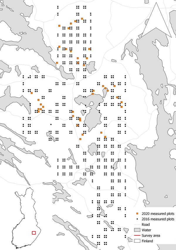
Fig 1. Locations of field plots used in 2016 and 2020. The 2016 data were used for the construction of a general diameter at breast height (DBH) model (Kukkonen et al. 2022) in option 1, and the 2020 data were used in the modelling and calibration of diameter at breast height and calculation of DBH in options 2 and 3.
The following attributes were computed for each plot: Stem count, basal area, diameter of the basal area median tree (DGM) and volume. DGM is an important measure related to the diameter distribution and it is a common input attribute in growth and yield models in Finland. It describes the diameter of the tree where the cumulative sum of the basal area of ascendingly ordered trees exceeds half of the sum of the basal areas of all trees. These attributes were calculated for Norway spruce, Scots pine and deciduous trees separately and together. Plot level attributes are shown in Table 1. For the evaluation of results, the plots were disaggregated into different development classes, three of which were present in the study area (Table 2). In our data, there were 1257 trees in plots classified as young, 1147 trees in plots classified as advanced, and 1088 trees plots classified as mature.
| Table 1. Descriptive statistics of the plot attribute data used in the modelling and calibration of diameter at breast height (DBH) and the calculation of the diameter of the basal area median tree (DGM) and volume. | ||||
| Average | Minimum | Maximum | Standard deviation | |
| DGM (cm) | 23.7 | 13.3 | 39.5 | 7.3 |
| Basal area (m2 ha–1) | 24.9 | 10.7 | 42.2 | 7.8 |
| Stem count (N ha–1) | 994.9 | 266.7 | 2155.6 | 515.5 |
| Height of the basal area median tree (m) | 21.1 | 8.8 | 30.0 | 5.5 |
| Volume (m3 ha–1) | 240.5 | 83.0 | 504.9 | 111.2 |
| Table 2. Development class criteria (Heikkilä 2016) used in the evaluation of results. | ||
| Class | Number of plots | Criteria |
| Young stands | 10 | Mean diameter at breast height 8–16 cm or dominant height ≥ 7 m (conifers) or ≥ 9 m (deciduous trees); mean age 0.4–0.8 × recommended rotation period 1 |
| Advanced stands | 13 | Mean diameter at breast height > 16 cm and < recommended regeneration diameter, mean age > 0.8 × recommended rotation period 1 |
| Mature stands | 16 | Diameter ≥ 18–25 cm, age 50–100 years |
| 1 Recommended rotation period describes the time period between two final fellings and depends on the situation and objectives (e.g. Pukkala 2007). Recommended rotation period used in this study is described in Ajosenpää (2009). | ||
UAV lidar data were collected in July 2020 under leaf-on conditions. Collection was made with an Avartek Boxer hybrid drone using a Riegl VUX-1 UAV scanner with an AP20 inertial measurement unit (IMU) (Table 3). All 39 sample plots were scanned from five south-north and five east-west flight lines. The UAV lidar data processing is described in Kukkonen et al. (2022), and the same data were used in this study.
| Table 3. Details of the hybrid drone Avartek Boxer, Riegl VUX-1 UAV scanner and AP20 inertial measurement unit (IMU) system used for data collection. | |
| Flight speed | 4 m s–1 |
| Flying altitude | 50 m |
| Pulse repetition frequency | 380 hHz |
| Pulse density | 3700 pulses m–2 |
| Scanning angle | 120° |
Individual trees were identified and segmented from lidar data with a watershed algorithm in combination with a canopy height model (CHM) as documented in Kukkonen et al. (2022). For all identified trees, height was estimated as the height of the highest lidar echo within a segment. Detected individual tree segments were linked with field measured trees based on observed spatial relationships within a three-dimensional space based on two criteria: 1) A field tree and a segment were required to be the closest neighbours to each other and 2) the distance between the field tree and the segment was ≤ 2 m (Kukkonen et al. 2022). During the segmentation process, a tree can be incorrectly segmented in two ways. A field-measured tree cannot be linked to any segment that causes a false negative or a non-existing tree might be segmented from a point cloud thereby causing a false positive (Wenkai et al. 2012; Kukkonen et al. 2022). This data included 63 identified false positives, which consisted of lidar-detected trees that were not linkable to any field-measured tree. These trees are hereafter referred to as false trees.
Kukkonen et al. (2022) constructed a general non-linear mixed-effects model fitted with data collected in 2016 from a wider area that surround our study site (Fig. 1). The 2016 dataset was collected by systematic sampling. It included 690 plots, and the trees in the plots were measured in the same way as in 2020. The Kukkonen et al. (2022) model was constructed based on height and diameter measurements. This model was used here in option 1.
2.2 Accuracy assessment
In this study, we calibrated our plot-level predictions by measuring tree variables in the field and using these measurements in model calibration. The accuracy of model predictions and calibrations was examined with DBH, DGM, tree volume and plot-level total volume per hectare. Calculations were carried out both with and without false trees. Although false trees could not be selected for calibration, they were included in the validation of results, because in real world applications, it is not known if a detected tree is a false tree. Volume was estimated for all trees, but false trees were ignored when the estimated and observed values were compared at the tree-level. However, false tree volumes were included in plot-level volume calculations. As the species of the detected trees was unknown, the volume of each tree was calculated three times, using the species-specific volume models for pine, spruce and birch (Laasasenaho 1982). Volume calculations were based on DBH, which was predicted in options 1–3, and on UAV-detected height. The final volumes were obtained by weighting the estimates by the total proportion of each species in the entire sample: 28.4% Scots pine, 47.0% Norway spruce and 24.6% deciduous trees. This was an estimate of the proportions of tree species, as the exact information on tree species proportions at the plot-level cannot be known (see Maltamo et al. 2003). These values were summed to produce a total volume estimate for each tree. Results are presented by development class and all together.
The accuracy between predicted and observed values was tested using root-mean-square error (RMSE, Eq. 1), relative RMSE (%RMSE), BIAS (Eq. 2) and relative BIAS (%BIAS). Both %RMSE and %BIAS were calculated by dividing RMSE and BIAS by the average of observed values and multiplying the result by 100.

![]() = observed value,
= observed value, ![]() = predicted value, n = the number of observations.
= predicted value, n = the number of observations.

![]() = observed value,
= observed value, ![]() = predicted value, n = the number of observations.
= predicted value, n = the number of observations.
All analyses were implemented using the R-software (R Core Team 2021) and Tidyverse-package (Wickham et al. 2019).
2.3 Modelling and calibration alternatives
Phases of three different modelling options are illustrated in Fig. 2.
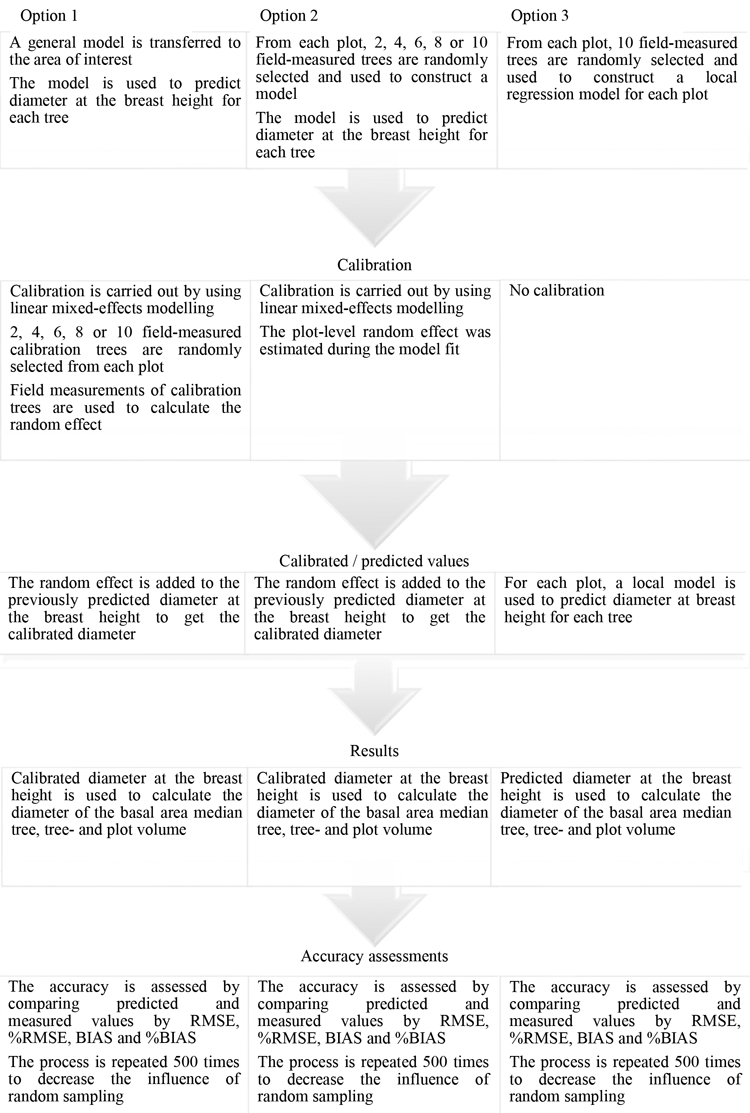
Fig 2. Flow chart describing the phases of the three different diameter at breast height (DBH) modelling and calibration options used in this study.
2.3.1 Calibration of the general mixed-effects model
We utilised a general DBH model that was refitted for this study to model and calibrate DBH. Kukkonen et al. (2022) formulated a mixed-effects model for the d/h relationship based on the wider area data collected in 2016. Species composition was assumed to follow the general composition of tree species in Finland. The model was re-fitted to the same data to obtain residual variances within (σe) and between (σb) plots. The model was transferred to the area of interest and the data collected in 2020 were used to calibrate this model. For all trees, DBH was calculated with this fixed model part using UAV-detected tree height instead of the field-measured estimate. The model was as follows:
![]()
![]() = predicted diameter at breast height (cm), h = field-measured tree height (m), bj = random parameter, see in Eq. 4.
= predicted diameter at breast height (cm), h = field-measured tree height (m), bj = random parameter, see in Eq. 4.
The model was calibrated using two, four, six, eight or ten calibration trees from each plot. False trees were excluded when calibration trees were selected. Calibration trees were selected randomly without replacement and their field-measured DBH-values were used to calculate the value of the random intercept parameter bj with the following equation (Eerikäinen 1999; Eq. 4):

where ![]() = variance between plots (cm),
= variance between plots (cm), ![]() = variance within plots (cm),
= variance within plots (cm), ![]() = the mean of field-measured tree diameters (cm),
= the mean of field-measured tree diameters (cm), ![]() = the mean of predicted tree diameters (cm), j = field plot.
= the mean of predicted tree diameters (cm), j = field plot.
Residual variances obtained from the model re-fitting were σb = 2.057 between plots and σe = 2.715 within plots.
Calibrated DBH-values were used to estimate DGM. Calibrated DBH-values together with UAV-detected tree heights were used to estimate tree- and plot-level volumes. The selection of calibration trees, the calculation of the random parameter and the calculation of predictions was repeated 500 times with each number of calibration trees to minimise the impact of random sampling. Calculations were carried out both with and without false trees.
2.3.2 Construction and calibration of local mixed-effects models
All measured trees from the 2020 field plots were used to fit new local non-linear mixed-effects models for the d/h relationship. These models were then applied so that the plot-level random effects that were estimated during the model fit were added to model fixed-part predictions. The difference from the previous scenario was that the data used for model construction was collected from a geographically smaller area, and so the number of measured trees was considerably smaller.
The models were formulated by randomly selecting two, four, six, eight or ten measured trees from each plot. False trees were excluded when trees were selected. R-software’s Linear and Nonlinear Mixed Effects Models (nlme) package (Pinheiro and Bates 2022) was used to estimate the parameters of the following model:
![]()
where DBH = diameter at breast height (cm), b1 and b2 = estimated fixed parameters, h = field-measured tree height (m), bj = estimated random parameters.
The fixed and random parts of model (5) were used to predict DBH for each tree using UAV-detected height instead of the field-measured estimate. Then DBH-values were used to estimate DGM, and DBH-values together with UAV-detected tree heights were used to estimate tree- and plot-level volumes.
The selection of the modelling trees, modelling and calibration of the random parameters, and the calculation of predictions was repeated 500 times with each sample size to minimise the impact of random sampling. The calculations were carried out both with and without false trees.
2.3.3 Formulation of plot-level models
A nonlinear regression model for DBH was formulated for each plot based on field-measured heights and DBH values of 10 randomly selected trees measured in 2020. In the model construction, ordinary nonlinear regression was used as the modelling data was not hierarchical. The model form was:
![]()
where d1.3 = diameter at breast height (cm), a and b = estimated model parameters, h = field-measured tree height (m).
For each tree in the plot, the plot-level model was used to calculate DBH using UAV-detected height. Then, DBH-values were used to estimate DGM, and DBH-values together with UAV-detected tree heights, were used to estimate tree- and plot-level volumes.
The selection of modelling trees, formulation of the models and calculation of predictions was repeated 500 times to minimise the impact of random sampling. The calculations were done carried out with and without false trees.
3 Results
3.1 Calibration of the general mixed-effects model
The general model (Eq. 3) was used to predict the DBH-values with and without false trees and %RMSE and %BIAS values associated with them were calculated (Fig. 3). In both cases, the DBH predictions improved moderately when the number of calibration trees was increased, and were better with no false trees in the calculations (%RMSE values ranged from 15.0–18.1 with no false trees and from 21.6–24.1 with false trees). In the predictions with no false trees, %BIAS decreased from 3.4% to 0.6%. However, with false trees, calibration turned %BIAS from a slight underestimation (0.7%) to a clear overestimation (–2.3%).
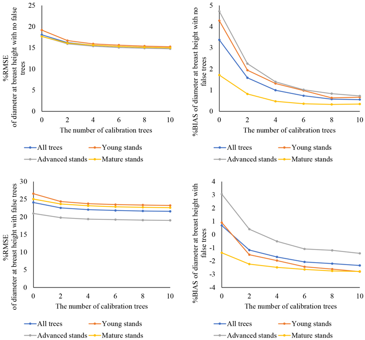
Fig 3. Prediction of diameter at breast height (DBH) with a general diameter/height model, calibration with field-measured trees and comparison with field measurements: relative root-mean-square error (%RMSE: left column) and relative BIAS (%BIAS: right column) with no false trees (upper row) and with false trees (lower row) are shown for the entire dataset and by development class.
The results of predicted variables’ %RMSE and %BIAS are illustrated in Fig. 4 (with no false trees), and Fig. 5 (with false trees). The corresponding absolute RMSE and BIAS values are presented in Suppl. files S2, S3, S4 and S5. Our results showed that the presence of false trees did not affect the results substantially. In the case of DGM, the predictions were practically the same (RMSE 7.4–13.1% with no false trees and 7.4–13.0% with false trees), while for plot-level volumes, the predictions with false trees (RMSE 24.7–28.3%) were almost the same as with no false trees (RMSE 25.1–29.3%).
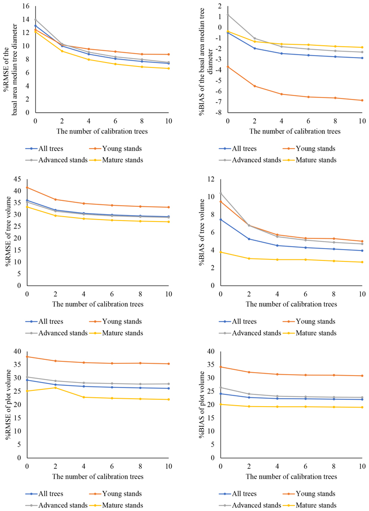
Fig 4. Prediction of diameter at breast height (DBH) with a general diameter/height model, calibration with field-measured trees, calculation of the diameter of the basal area median tree (DGM), tree and plot volumes and comparison with field measurements: relative root-mean-square error (%RMSE: left column) and relative BIAS (%BIAS: right column) with no false trees are shown for the entire dataset and by development class.
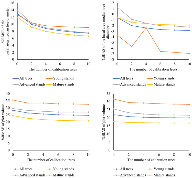
Fig. 5. Prediction of diameter at breast height (DBH) with a general diameter/height model, calibration with field-measured trees, calculation of the diameter of the basal area median tree (DGM), tree and plot volumes, and comparison with field measurements: relative root-mean-square error (%RMSE: left column) and relative BIAS (%BIAS: right column) with false trees are shown for the entire dataset and by development class.
Calibration decreased the %RMSE values in all cases when compared with the predictions obtained with the fixed part of the general model only (i.e. the number of calibration trees = 0). As the number of calibration trees increased, the predictions improved. Especially with DGM, the largest improvement in predictions was observed with two (10% with and without false trees) to four (8.8% with and without false trees) calibration trees, when compared with the predictions obtained using only the fixed part (13.1% with no false trees and 13.0% with false trees). For volume predictions, the greatest improvement in predictions was observed with two calibration trees. After that, increasing the number of calibration trees did not have a notable impact on the results.
When the effect of calibration was examined by development class, the RMSE value was the poorest in the young stands. However, in this case, calibration seemed to improve DGM predictions (from 12.4% to 8.8–10.2% with no false trees and from 12.7% to 9.1–10.4% with false trees). The best RMSE value was achieved in the mature stands (6.6% with no false trees and using 10 calibration trees). In this case, the calibration did not seem to have as large effect as in the other classes.
For BIAS, it seemed that both tree- and plot-level volumes were somewhat underestimated, but calibration decreased the BIAS (from 7.5% to 4.0–5.3% for tree-level volume, from 24.1% to 22.0–22.7% with no false trees and from 22.1% to 20.0–20.8% with false trees for plot level volume. In the case of DGM, the effect of an increasing number of calibration trees was the opposite and BIAS values increased when the number of calibration trees increased (from –0.5% to –2.0 – –2.9%). All %BIAS values except uncalibrated predictions in the advanced stands, were negative, which indicated that the model overestimated DGM values.
3.2 Local mixed-effects models and calibration
The results of the DBH predictions calculated with models that were constructed based on the study area data are illustrated In Fig. 6 both with and without false trees. Improvement in DBH predictions was minor when the number of trees was increased (RMSE% 15.3–16.7 with no false trees and 21.7–23.0% with false trees). With no false trees, BIAS values increased slightly (from 2.3% to 2.6%) while with false trees it decreased (from –0.6% to –0.1%) when the number of trees increased.
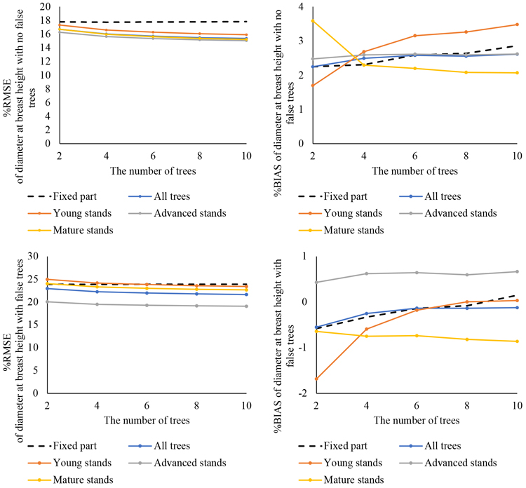
Fig 6. Prediction of diameter at breast height (DBH) with newly constructed diameter/height models, calibration and comparison with field measurements: relative root-mean-square error (%RMSE: left column) and relative BIAS (%BIAS: right column) with no false trees (upper row) and with false trees (lower row) are shown for the entire dataset and by development class. The fixed part of the model shows the performance for all trees without calibration.
The predicted DBH-values are illustrated in Fig. 7 (with no false trees) and in Fig. 8 (with false trees). Corresponding absolute RMSE and BIAS values associated with the predictions are presented in Suppl. files S6, S7, S8 and S9. For DGM, the addition of false trees to the data did not influence the results (RMSE% 10.5–6.9% with no false trees and 10.6–7.0% with false trees). However, the data that included false trees produced somewhat better results for plot-level volumes (RMSE% 29.5–28.7% with no false trees and 28.2–27.1% with false trees).
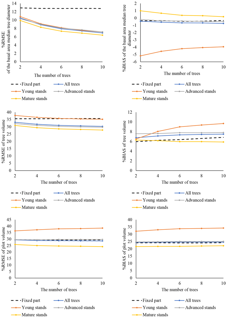
Fig. 7. Prediction of diameter at breast height (DBH) with newly constructed diameter/height models, calibration, calculation of the diameter of the basal area median tree (DGM), tree and plot volumes and comparison with field measurements: relative root-mean-square error (%RMSE: left column) and relative BIAS (%BIAS: right column) with no false trees are shown forthe entire dataset and by development class. The fixed part of the model shows the performance for all trees without calibration.
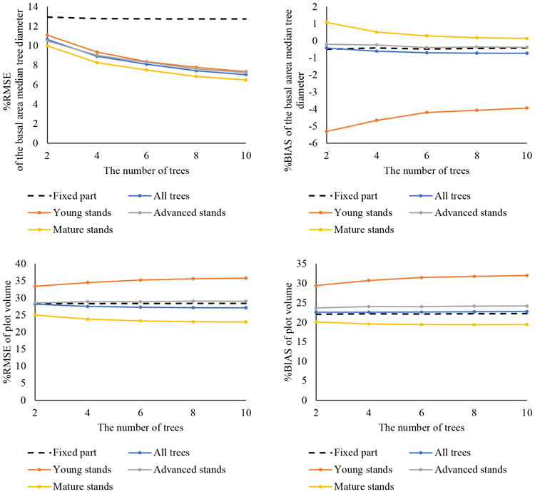
Fig. 8. Prediction of diameter at breast height (DBH) with newly constructed diameter/height models, calibration, calculation of the diameter of the basal area median tree (DGM), tree and plot volumes and comparison with field measurements: relative root-mean-square error (%RMSE: left column) and relative BIAS (%BIAS: right column) with false trees are shown for the entire dataset and by development class. The fixed part of the model shows the performance for all trees without calibration.
Models were constructed with two, four, six, eight and ten trees. The predictions were calculated with the fixed parts of these models and compared with predictions obtained from calibration with the random effects. The predictions made with the fixed parts only were practically the same regardless of the number of trees used in model construction. The %RMSE and %BIAS values for all trees with the fixed part of the model are shown in Figs. 7 and 8. For young stands, advanced stands and mature stands with no false trees, the fixed part values were approximately 14%, 13% and 12% for DGM, 40%, 34% and 33% for tree-level volume and 35%, 28% and 25% for plot-level volume, respectively (Suppl. files S7, S8 and S9). With false trees, the corresponding fixed part values were 14%, 13% and 12% for DGM and 32%, 28% and 25% for plot level volume. As with the general model, calibration improved the predictions of all variables with regard to %RMSE. However, the observed improvement in the predictions as the number of calibration trees was increased was not as notable as with the transferred model. Increasing the number of calibration trees from two to four improved the results slightly more than when the number of trees increased beyond four. The greatest changes in predictions were observed with DGM. In the case of tree- and plot-level volumes, the changes were minor.
When the predictions were examined for each development class, model performance in the young stands was the weakest. For plot-level volumes, the predictions disimproved as the number of modelling trees increased (RMSE% 36.4% to 38.5% with no false trees and from 33.4% to 35.8% with false trees). In the case of DGM and volume, the best prediction accuracy was observed in the mature stands. In the advanced stands, the RMSE values associated with plot volume seemed to stay at the same level regardless of the number of the modelling trees (29.6–29.8% with no false trees and 28.6–29% with false trees).
As with the general model, BIAS value was negative in the case of DGM and increased as the number of trees increased (from –0.4% to –0.7% with no false trees and from –0.4% to –0.7% with false trees when the model was calibrated). In young stands, the effect was opposite and increasing the number of trees decreased the BIAS values (from –5.2% to –3.9% with no false trees and from –5.3% to –3.9% with false trees). Tree-level volume BIAS values seemed to stay relatively constant as the number of trees increased (from 6.8% to 7.5%), except for the young stands where it increased (from 6.5% to 9.7%). In the case of plot-level volumes, increasing the number of calibration trees barely affected BIAS (24.5–24.7% with no false trees and 22.6–22.7% with false trees). Plot volume predictions were underestimated whereas DGM predictions were overestimated, similar to the general model.
3.3 Plot-level regression models
The RMSE values associated with the plot-level model predictions showed that the inclusion of false trees in the dataset had only a minor effect on the results (Table 4, Table 5). The results were slightly better in the case of DGM, with no false trees, and with false trees in the case of plot volume. As in the previous stages, the predictions were generally weaker in young stands.
| Table 4. Prediction of diameter at breast height (DBH) with plot-level diameter/height models, calculation of the diameter of the basal area median tree (DGM), tree volume and plot volumes, and comparison of the results with field measurements: absolute (RMSE) and relative root-mean-square error (%RMSE) and absolute (BIAS) and relative BIAS (%BIAS) values with no false trees are shown for the entire dataset and by development class. | ||||
| RMSE | %RMSE | BIAS | %BIAS | |
| DBH | ||||
| All | 3.40 cm | 15.26 | 0.75 | 3.45 |
| Young stands | 2.64 cm | 16.28 | 0.73 | 4.48 |
| Advanced stands | 3.00 cm | 15.16 | 0.61 | 3.15 |
| Mature stands | 4.19 cm | 14.72 | 0.88 | 3.04 |
| DGM | ||||
| All | 1.51 cm | 6.37 | –0.14 | –0.57 |
| Young stands | 1.11 cm | 6.88 | –0.39 | –2.40 |
| Advanced stands | 1.44 cm | 7.00 | –0.09 | –0.42 |
| Mature stands | 1.71 cm | 5.54 | –0.02 | –0.05 |
| Tree-level volume | ||||
| All | 137.40 m3 | 30.20 | 38.25 | 8.63 |
| Young stands | 62.13 m3 | 34.99 | 21.32 | 11.52 |
| Advanced stands | 91.24 m3 | 30.03 | 23.53 | 8.21 |
| Mature stands | 221.94 m3 | 27.34 | 60.78 | 7.16 |
| Total volume | ||||
| All | 72.31 m3 ha–1 | 30.07 | 61.48 | 25.56 |
| Young stands | 64.69 m3 ha–1 | 40.46 | 56.81 | 35.53 |
| Advanced stands | 55.70 m3 ha–1 | 30.84 | 46.16 | 25.56 |
| Mature stands | 87.06 m3 ha–1 | 25.64 | 76.84 | 22.63 |
| Table 5. Prediction of diameter at breast height (DBH) with plot-level diameter/height models, calculation of the diameter of the basal area median tree (DGM), tree- and plot-volumes, and comparison of the results with field measurements: absolute (RMSE) and relative root-mean-square error (%RMSE) and absolute (BIAS) and relative BIAS (%BIAS) values with false trees are shown for the entire dataset and by development class. | ||||
| RMSE | %RMSE | BIAS | %BIAS | |
| DBH | ||||
| All | 4.74 cm | 22.11 | 0.05 | 0.33 |
| Young stands | 3.60 cm | 23.34 | 0.22 | 1.29 |
| Advanced stands | 3.68 cm | 19.52 | 0.19 | 0.91 |
| Mature stands | 6.31 cm | 23.44 | –0.18 | –0.74 |
| DGM | ||||
| All | 1.71 cm | 7.22 | –0.15 | –0.64 |
| Young stands | 1.12 cm | 6.95 | –0.39 | –2.38 |
| Advanced stands | 1.43 cm | 6.92 | –0.04 | –0.20 |
| Mature stands | 2.04 cm | 6.61 | –0.10 | –0.31 |
| Total volume | ||||
| All | 68.57 m3 ha–1 | 28.51 | 57.02 | 23.71 |
| Young stands | 60.47 m3 ha–1 | 37.82 | 53.22 | 33.29 |
| Advanced stands | 54.60 m3 ha–1 | 30.23 | 44.59 | 24.69 |
| Mature stands | 81.97 m3 ha–1 | 24.14 | 69.51 | 20.47 |
The BIAS values mostly followed the pattern of RMSE; less in the development classes where RMSE values were smaller. An exception was DGM in the young stands, where the BIAS value was notably larger than in the other cases. For DGM, the BIAS values were negative i.e. the predictions were underestimated. The tree- and plot-level volumes were similarly underestimated as with the general model and the newly constructed random-effects models.
4 Discussion
The objective of this work was to compare the calibration of a general mixed-effects model with local models constructed for an area of interest. With both the general and local mixed-effects models, calibration improved the RMSE values of all predicted variables. The greatest improvement was seen when two calibration trees were used rather than the fixed part of the model only. Further increases in the number of calibration trees improved the results although the effect was not as substantial as with two trees. Similar results have been observed in previous studies (Maltamo et al. 2012; Korhonen et al. 2019). Calibration improved the results for the general mixed-effects model more than for the locally constructed models. This seems logical as our local models were based on the data collected directly from the study area, and therefore the models directly described the study area data. The regression models constructed at the plot-level produced very similar results as the mixed-effects models. In this case, each model described only one plot and the variation in this plot enabled accurate estimates.
One advantage of the transferred model was that it was constructed based on a large data set. In this study, the models fitted locally in the study area contained 78–390 trees. This may lead to errors in model formulation if the selected sample of trees gives an unrepresentative sample of the tree population. With the transferred model, the prediction accuracy was at the same level as the local mixed-effects or regression models. This suggests that the use of a transferred model is possible and that the laborious task of field data collection for a local model can be avoided by calibration. In that case, only a small number of field measurements from the study area are required. As the greatest improvement in predictions was obtained with just two calibration trees, from the perspective of field measurements, this may be a good option as a reasonable accuracy can be obtained with minor effort. However, from the perspective of prediction accuracy, the RMSE value is not yet at the required level, and so more calibration trees may be needed.
The number of false trees created by unsuccessful tree detection was relatively small (n = 63) and their inclusion in the analyses had little effect on the results. However, as false trees are unavoidable in individual tree inventories, they were retained in the analyses. There are techniques to correct for errors related to false trees (Kostensalo et al. 2023), but these were not used in this study. The plot volume predictions calculated with false trees were even slightly better than the predictions where they were not included. The reason was that identification of all trees from remotely sensed data is not possible and therefore volume is typically underestimated. As false trees also receive a volume estimate, the increased total volume brings the estimated values closer to the true volume. This effect is strongly dependent on the forest structure and is typically reasonably small. However, in some mature plots the number of false trees might be large and the number of missed trees might be small, which could cause volume overestimation, which will immediately influence the overall BIAS. In our plots, the false tree volumes typically compensated 0%–59% of the volume of undetected trees, but in one plot this number was 239% due to the large number of false trees.
We observed that the model performance was considerably weaker in young stands compared to mature and advanced stands. Typically, individual tree detection performs better in mature stands than in denser young stands, where most segmentation methods (e.g the watershed algorithm used in this study) often fail to detect small trees growing under larger ones. It has also been observed that not every small tree may be detected, even with high-density UAV lidar data (Liang et al. 2019). This leads to a lack of small-diameter trees when constructing local diameter models (options 2 and 3 in this study), which can cause errors in predictions. In mature stands, the lack of small-diameter trees might be highlighted, as small trees growing underneath larger ones are not easily detected. In young stands, the height differences are smaller but the stem count is greater, which has been shown to be problematic in automatic tree detection (Jeronimo et al. 2018).
Our models overestimated DGM, and the increase in the number of calibration trees led to increased overestimation. The BIAS values associated with tree- and plot-level volumes suggest that the volumes were underestimated. In the mature stands, the predictions were underestimated more than in the young stands. In older trees, height growth slows down but diameter growth continues. The models used in our study only considered height when predicting diameter, which may lead to underestimated diameters for old trees. The volume estimations of undetected small trees were missing from the estimation. However, their combined total volume is very small and not likely to affect the results substantially.
Previous studies conducted in Finland have shown that the transfer of area-based models especially in a north-south direction, can cause errors in predictions, although calibration with regional measurements can improve model performance (Kotivuori et al. 2016). In our study, the general model was transferred from a geographically adjacent area, which may have produced better results. In contrast to earlier model calibration studies (Maltamo et al. 2012; Korhonen et al. 2019), our results seem somewhat more accurate. However, model formulations in previous studies were more complex, which suggests that model transfer and calibration perform better when the model is simple. Different forest structures and differences between ALS-devices might also have an impact on the results, although calibration appeared to reduce the associated errors (Kotivuori et al. 2016).
In this study, the calibration trees were randomly selected from the field data. However, in practice calibration trees would be intentionally selected. In that case, the trees are not necessarily selected objectively, and small and large trees have equal probability to be selected. On the other hand, subjectively selected calibration trees may also lead to better performance than observed here e.g, if trees with an unusual DBH-height relationship are ignored. Incorrect tree detection may also cause problems in the selection of the calibration trees. If the calibration trees are measured in the field while the UAV-data is being collected, the measured trees may not be identified from the remotely sensed data afterwards. On the other hand, linking field-measured and UAV-detected trees might be difficult or even impossible.
5 Conclusions
The objective of this study was to compare the predictions produced by a general model and newly constructed models. Models were constructed with UAV-data and were calibrated with a small number of field measurements. Predictions were carried out by using a calibrated general mixed-effects model, by the construction of new mixed-effects models that were calibrated, and by the construction of plot-level regression models. Our results showed that the differences in predictions between the various model options were minor. Using a general model with a small number of calibration measurements, which can be measured during UAV data acquisition, seems to be a useful option to reduce the costs and workload associated with forest inventories.
Declaration of openness of research materials, data, and code
The data used in this study are not openly available. Codes used in the study can be made available by reasonable request by e-mail to the first author.
Author contributions
JJ: Data analysis, Interpretation of results, Writing – original draft.
LK: Conceptualisation, Writing – revisions, Supervision.
MK: Data acquisition (expert assessment), Writing – revisions.
PP: Data acquisition (expert assessment), Writing – revisions.
MM: Conceptualisation, Writing – revisions, Supervision.
Funding
This work was supported by the Finnish Flagship Programme of the Academy of Finland for the Forest–Human–Machine Interplay — Building Resilience, Redefining Value Networks and Enabling Meaningful Experiences (UNITE) project (decision numbers 337127, 337655 and 357909), led by Heli Peltola at the School of Forest Sciences, University of Eastern Finland, by the Academy of Finland through the project Unmanned Aerial Vehicles in Forest Remote Sensing (351525) and Is climate smart forestry a utopia if the preferences of landowners are not considered? (352782).
References
Ajosenpää T (2009) Solmu-maastotyöopas 3rd edition. [Solmu -field work quide]. Metsätalouden kehittämiskeskus Tapio. Metsäkustannus, Helsinki.
Bondell HD, Krishna A, Ghosh SK (2010) Joint variable selection for fixed and random effects in linear mixed-effects models. Biometrics 66: 1069–1077. https://doi.org/10.1111/j.1541-0420.2010.01391.x.
Calama R, Montero G (2004) Interregional nonlinear height–diameter model with random coefficients for stone pine in Spain. Can J Forest Res 34: 150–163. https://doi.org/10.1139/x03-199.
Chen X, Jiang K, Zhu Y, Wang X, Yun T (2021) Individual tree crown segmentation directly from UAV-borne LiDAR data using the PointNet of deep learning. Forests 12, article id 131. https://doi.org/10.3390/f12020131.
Chianucci F, Disperati L, Guzzi D, Bianchini D, Nardino V, Lastri C, Rindinella A, Corona P (2016) Estimation of canopy attributes in beech forests using true colour digital images from a small fixed-wing UAV. Int J Appl Earth Obs 47: 60–68. https://doi.org/10.1016/j.jag.2015.12.005.
Dainelli R, Toscano P, Di Gennaro SF, Matese A (2021) Recent advances in unmanned aerial vehicle forest remote sensing – a systematic review. Part I: a general framework. Forests 12, article id 327. https://doi.org/10.3390/f12030327.
Eerikäinen K (1999) Random parameter model for the relationship between stand age and tree height in Zambia. In: Pukkala T, Eerikäinen K (eds) Growth and yield modelling of tree plantations in South and East Africa. University of Joensuu, Faculty of Forestry, Research Notes 97: 153–165.
Fahlstom P, Gleason T (2012) Introduction to UAV systems 4th edition. John Wiley & Sons, Chichester. https://doi.org/10.1002/9781118396780.
Guimarães N, Pádua L, Marques P, Silva N, Peres E, Sousa JJ (2020) Forestry remote sensing from unmanned aerial vehicles: a review focusing on the data, processing and potentialities. Remote Sens-Basel 12, article id 1046. https://doi.org/10.3390/rs12061046.
Heikkilä J (2016) Maastotyöohje Liperi 2016. [Field work instruction Liperi 2016]. Finnish Forest Centre.
Hui Z, Li N, Xia Y, Cheng P, He Y (2021) Individual tree extraction from UAV lidar point clouds based on self-adaptive mean shift segmentation. ISPRS Ann Photogramm Remote Sens Spatial Inf Sci V-1-2021: 25–30. https://doi.org/10.5194/isprs-annals-V-1-2021-25-2021.
Hyyppä E, Kukko A, Kaartinen H, Xiaowei Y, Muhojoki J, Hakala T, Hyyppä J (2022) Direct and automatic measurements of stem curve and volume using a high-resolution airborne laser scanning system. Sci Remote Sens 5, article id 100050. https://doi.org/10.1016/j.srs.2022.100050.
Jeronimo SMA, Kane VR, Churchill DJ, McGaughey RJ, Franklin JF (2018) Applying LiDAR individual tree detection to management of structurally diverse forest landscapes. J For 116: 336–346. https://doi.org/10.1093/jofore/fvy023.
Kalliovirta J, Tokola T (2005) Functions for estimating stem diameter and tree age using tree height, crown width and existing stand database information. Silva Fenn 39: 227–248. https://doi.org/10.14214/sf.386.
Karjalainen T, Korhonen L, Packalen P, Maltamo M (2019) The transferability of airborne laser scanning based tree-level models between different inventory areas. Can J Forest Res 49: 228–236. https://doi.org/10.1139/cjfr-2018-0128.
Korpela I, Tuomola T, Välimäki E (2007) Mapping forest plots: an efficient method combining photogrammetry and field triangulation. Silva Fenn 41: 457–469. https://doi.org/10.14214/sf.283.
Kostensalo J, Mehtätalo L, Tuominen S, Packalen P, Myllymäki M (2023) Recreating structurally realistic tree maps with airborne laser scanning and ground measurements. Remote Sens Environ 298, article id 113782. https://doi.org/10.1016/j.rse.2023.113782.
Kotivuori E, Korhonen L, Packalen P (2016) Nationwide airborne laser scanning based models for volume, biomass and dominant height in Finland. Silva Fenn 50, article id 1567. https://doi.org/10.14214/sf.1567.
Kotivuori E, Kukkonen M, Mehtätalo L, Maltamo M, Korhonen L, Packalen P (2020) Forest inventories for small areas using drone imagery without in-situ field measurements. Remote Sens Environ 237, article id 111404. https://doi.org/10.1016/j.rse.2019.111404.
Kukkonen M, Kotivuori E, Maltamo M, Korhonen L, Packalen P (2021a) Volumes by tree species can be predicted using photogrammetric UAS data, Sentinel-2 images and prior field measurements. Silva Fenn 55, article id 10360. https://doi.org/10.14214/sf.10360.
Kukkonen M, Maltamo M, Korhonen L, Packalen P (2021b) Fusion of crown and trunk detections from airborne UAS based laser scanning for small area forest inventories. Int J Appl Earth Obs 100, article id 102327. https://doi.org/10.1016/j.jag.2021.102327.
Kukkonen M, Maltamo M, Korhonen L, Packalen P (2022) Evaluation of UAS LiDAR data for tree segmentation and diameter estimation in boreal forests using trunk and crown based methods. Can J Forest Res 52: 674–684. https://doi.org/10.1139/cjfr-2021-0217.
Kuželka K, Slavík M, Surový P (2020) Very high density point clouds from UAV laser scanning for automatic tree stem detection and direct diameter measurement. Remote Sens-Basel 12, article id 1236. https://doi.org/10.3390/rs12081236.
Laasasenaho J (1982) Taper curve and volume functions for pine, spruce and birch. Communicationes instituti forestalis Fenniae 108. Finnish Forest Research Institute (Metla), Helsinki. http://urn.fi/URN:ISBN:951-40-0589-9.
Liang X, Wang Y, Pyörälä J, Lehtomäki M, Yu X, Kaartinen H, Kukko A, Honkavaara E, Issaoui AEI, Nevalainen O, Vaaja M, Virtanen J-P, Katoh M, Deng S (2019) Forest in situ observations using unmanned aerial vehicle as an alternative of terrestrial measurements. For Ecosyst 6, article id 20. https://doi.org/10.1186/s40663-019-0173-3.
Maltamo M, Tokola T, Lehikoinen M (2003) Estimating stand characteristics by combining single tree pattern recognition of digital video imagery and a theoretical diameter distribution model. Forest Sci 49: 98–109.
Maltamo M, Packalén P, Peuhkurinen J, Suvanto A, Pesonen A, Hyyppä J (2007) Experiences and possibilities of ALS based forest inventory in Finland. In: Rönnholm P, Hyyppä H, Hyyppä J (eds) Proceedings of ISPRS Workshop Laser Scanning 2007 and Silvilaser 2007, September 12–14, 2007, Finland. Int Arch Photogramm Remote Sens XXXVI (Part 3/W52): 270–279.
Maltamo M, Mehtätalo L, Vauhkonen J, Packalén P (2012) Predicting and calibrating tree size and quality attributes by means of airborne laser scanning and field measurements. Can J Forest Res 42: 1896–1907. https://doi.org/10.1139/x2012-134.
Mehtätalo L, Lappi J (2020) Linear mixed-effects models. Biometry for forestry and environmental data with examples in R 1st edition. CRC press, Boca Raton and Oxon. https://doi.org/10.1201/9780429173462.
Mehtätalo L, de-Miguel S, Gregoire T (2015) Modeling height-diameter curves for prediction. Can J Forest Res 45: 826–837. https://doi.org/10.1139/cjfr-2015-0054.
National Land Survey of Finland (2023a) General map 1:1 M. https://tiedostopalvelu.maanmittauslaitos.fi/tp/kartta?lang=en. Accessed 14 March 2023.
National Land Survey of Finland (2023b) Municipal division 1:10 000. https://tiedostopalvelu.maanmittauslaitos.fi/tp/kartta?lang=en. Accessed 14 March 2023.
Oliveira RA, Khoramshahi E, Suomalainen J, Hakala T, Viljanen N, Honkavaara E (2018) Real-time and post-processed georeferencing for hyperspectral drone remote sensing. Int Arch Photogramm Remote Sens Spatial Inf Sci XLII-2: 789–795. https://doi.org/10.5194/isprs-archives-XLII-2-789-2018.
Pádua L, Vanko J, Hruška J, Adão T, Sousa JJ, Peres E, Morais R (2017) UAS, sensors, and data processing in agroforestry: a review towards practical applications. Int J Remote Sens 38: 2349–2391. https://doi.org/10.1080/01431161.2017.1297548.
Pinheiro J, Bates D (2022) R Core Team. Nlme: linear and nonlinear mixed effects models. R package version 3.1-158. https://CRAN.R-project.org/package=nlme. Accessed 27 February 2023.
Pukkala T (2007) Metsäsuunnittelun menetelmät. [The methods of forest planning]. Gummerus, Vaajakoski.
R Core Team (2021) R: a language and environment for statistical computing. R Foundation for Statistical Computing, Vienna, Austria. https://www.R-project.org/. Accessed 27 February 2023.
Räty J, Packalen P, Kotivuori E, Maltamo M (2020) Fusing diameter distributions predicted by an area-based approach and individual-tree detection in coniferous-dominated forests. Can J Forest Res 50: 113–125. https://doi.org/10.1139/cjfr-2019-0102.
Toivonen J, Korhonen L, Kukkonen M, Kotivuori E, Maltamo M, Packalen P (2021) Transferability of ALS based forest attribute models when predicting with drone-based image point cloud data. Int J Appl Earth Obs 103, article id 102484. https://doi.org/10.1016/j.jag.2021.102484.
Tompalski P, White JC, Coops NC, Wulder MA (2019) Demonstrating the transferability of forest inventory attribute models derived using airborne laser scanning data. Remote Sens Environ 227: 110–124. https://doi.org/10.1016/j.rse.2019.04.006.
Vandendaele B, Fournier RA, Vepakomma U, Pelletier G, Lejeune P, Martin-Ducup O (2021) Estimation of northern hardwood forest inventory attributes using UAV laser scanning (ULS): transferability of laser scanning methods and comparison of automated approaches at the tree- and stand-level. Remote Sens-Basel 13, article id 2796. https://doi.org/10.3390/rs13142796.
Wenkai L, Qinghua G, Marek KJ, Maggi K (2012) A new method for segmenting individual trees from the lidar point cloud. Photogramm Eng Rem S 78: 75–84. https://doi.org/10.14358/PERS.78.1.75.
Wickham H, Averick M, Bryan J, Chang W, McGowan LD, François R, Grolemund G, Hayes A, Henry L, Hester J, Kuhn M, Pedersen TL, Miller E, Bache SM, Müller K, Ooms J, Robinson D, Seidel DP, Spinu V, Takahashi K, Vaughan D, Wilke C, Woo K, Yutani H (2019). Welcome to the tidyverse. J Open Source Softw 4, article id 1686. https://doi.org/10.21105/joss.01686.
Total of 43 references.
