Ole Martin Bollandsås  ,
Terje Gobakken,
Erik Næsset,
Bjørn-Eirik Roald,
Hans Ole Ørka
,
Terje Gobakken,
Erik Næsset,
Bjørn-Eirik Roald,
Hans Ole Ørka
Impact of point cloud matching on precision and accuracy in area-based forest inventories
Bollandsås O. M., Gobakken T., Næsset E., Roald B.-E., Ørka H. O. (2025). Impact of point cloud matching on precision and accuracy in area-based forest inventories. Silva Fennica vol. 59 no. 3 article id 25002. https://doi.org/10.14214/sf.25002
Highlights
- The quality of forest attribute models based on variables obtained from image matching point clouds constructed using different software packages was analyzed
- Different software yielded no significant differences between models
- A comparison showed that models based on variables calculated from airborne laser scanning point clouds were superior.
Abstract
Reliable forest inventory methods are important for informed management. The current study compared the quality of forest attribute models based on metrics from image matching point clouds, generated using various software packages, with those based on metrics from airborne laser scanning. The field- and remotely sensed data used in the analyses were collected as part of an operational forest management inventory in Norway. Results indicate that models based on point cloud data from airborne laser scanning (ALS) consistently produced smaller root mean square error values, demonstrating superior accuracy in capturing complex forest structures compared to models using image matching point clouds. While image matching offers advantages such as lower costs and broader area coverage, this data source primarily represents canopy surfaces, which complicate its use in inventories requiring detailed canopy information. Statistical analyses revealed no significant differences in model performance among various image matching software, but all being inferior to ALS. The study emphasizes the importance of selecting the appropriate source of remotely sensed data based on specific inventory needs.
Keywords
airborne laser scanning;
remote sensing;
aerial images
-
Bollandsås,
Faculty of Environmental Sciences and Natural Resource Management, Norwegian University of Life Sciences, Box 5003, 1430 Ås, Norway
 https://orcid.org/0000-0002-1231-7692
E-mail
ole.martin.bollandsas@nmbu.no
https://orcid.org/0000-0002-1231-7692
E-mail
ole.martin.bollandsas@nmbu.no
-
Gobakken,
Faculty of Environmental Sciences and Natural Resource Management, Norwegian University of Life Sciences, Box 5003, 1430 Ås, Norway
https://orcid.org/0000-0001-5534-049X
E-mail
terje.gobakken@nmbu.no
- Næsset, Faculty of Environmental Sciences and Natural Resource Management, Norwegian University of Life Sciences, Box 5003, 1430 Ås, Norway E-mail erik.naesset@nmbu.no
- Roald, Faculty of Environmental Sciences and Natural Resource Management, Norwegian University of Life Sciences, Box 5003, 1430 Ås, Norway E-mail bjorn-eirik.roald@nmbu.no
-
Ørka,
Faculty of Environmental Sciences and Natural Resource Management, Norwegian University of Life Sciences, Box 5003, 1430 Ås, Norway
https://orcid.org/0000-0002-7492-8608
E-mail
hans-ole.orka@nmbu.no
Received 3 February 2025 Accepted 1 November 2025 Published 18 November 2025
Views 15680
Available at https://doi.org/10.14214/sf.25002 | Download PDF

Supplementary Files
1 Introduction
Forests ecosystems play a crucial role globally, influencing climate, biodiversity, and providing essential resources. Accurate and precise forest inventories are vital for sustainable forest management, as they enable informed decision-making regarding ecosystem services, such as harvesting, conservation, and carbon sequestration. During the last decades, forest management inventories in numerous countries all over the world have relied on remotely sensed data, in particular airborne laser scanning (ALS) (Maltamo et al. 2014). ALS data have mostly been utilized according to the area-based approach (Næsset 2002b) in which predictive models for volume, dominant and mean height, basal area and other stand descriptive attributes are calibrated using field observations from sample plots. The models are based on metrics calculated from the height distributions of ALS echoes reflected from the spatial extents of the field plots, metrics representing both the height and density of the forest. Estimates of the forest attributes on stand level are obtained by first applying the models for prediction on grid cells tessellating the entire area of interest and then aggregating the predictions that fall within the respective stand borders. The size of these grid cells is generally the same size as the field plots used for model calibration because the explanatory variables calculated from point clouds are scale dependent.
While ALS remains prevalent in forest management inventories, the significance of information from aerial imaging persists, with a historical presence in forest mapping dating back to pre-World War II (Standish 1945; Spurr 1952; Loetsch et al. 1964; Korpela 2004). For example, two-dimensional applications, such as tree species determination and stand delineation (White et al. 2016), have been operational for many decades. With the rapid rise of digital computing, acquiring three-dimensional data automatically through the processing of overlapping images became feasible (Næsset 2002a; St‐Onge et al. 2008). Studies that have compared the utility of point clouds generated using image matching and ALS for forest information purposes (Järnstedt et al. 2012; Gobakken et al. 2015; White et al. 2018) have consistently indicated that estimates obtained from image matching data are less precise and accurate than those obtained through ALS. Challenges associated with image matching include variable quality and resolution of imagery, all of which impact the quality of generated point clouds. Furthermore, constructing accurate digital terrain models (DTM) using image matching presents challenges. As a result, it is usually necessary to acquire a DTM from an alternative source before utilizing image matching data for predicting tree heights and timber volumes. Despite these challenges, image matching offers advantages such as lower acquisition costs compared to ALS, the ability to cover larger areas in single acquisitions, and the potential for obtaining retrospective forest information by matching historical images. The trade-offs between precision and cost-effectiveness make image matching a viable alternative for certain applications in forest inventory, underscoring the need for a more nuanced understanding of its strengths and limitations within the broader context of remote sensing technologies.
There exist many commercial software packages that can be used to construct point clouds from the aerial photographs by means of image matching. Studies (Alidoost and Arefi 2017; Harshit et al. 2023) have shown that the attributes of the resulting point clouds may be dependent on the software used. For instance, Alidoost and Arefi (2017) investigated and compared the performances of four different software packages for generating high density point clouds and digital surface models from images captured by unmanned aerial systems over an archeological site. They applied both visual and geometric assessments, and results showed that the software producing the fewest points was also the one that produced the most accurate surface model. In the study by Harshit et al. (2023) four different open-source software packages were compared to two commercial software packages. Their focus was to review the recent development of open-source software by comparing results to those obtained by using commercial products. Using a dataset covering a combination of buildings and urban vegetation, they found point cloud differences that could be attributed to software. Furthermore, Niederheiser et al. (2016) compared point clouds derived from terrestrial images of a rock face surrounded by sparse vegetation using different software. They noted that image input and matching software had greater impact on the point cloud properties over vegetation compared to those representing the smoother rock face.
While the choice of software for generating point clouds influences their properties, such as the number and distribution of points, these differences do not inherently denote superiority or inferiority in the context of area-based forest inventory, carried out in the form that is described above. Since the properties of each point cloud represented by statistical metrics are regressed against ground reference observations, estimates that result from aggregating subsequent model predictions over stands are often subject to small or negligible systematic errors irrespective of the source of the auxiliary data. However, this assumption is valid only if the prediction model is built on sample data that accurately reflects the overall relationship between the auxiliary data and the response for the entire population subject to analysis.
The advantages related to the acquisition of image matching point clouds as discussed above, have been decisive for that operational forest inventories sometimes have chosen image matching over ALS. However, with a multitude of possible combinations of image qualities, software for processing, and settings in the matching procedures, care should be taken before relying on image matching point clouds for forest inventory purposes. Although there are several studies that have tested and compared the performance of image matching versus ALS, there are, to the best of our knowledge, no studies that at the same time have studied the effect of processing the same set of aerial images using different software. Knowledge of possible adverse effects due to processing is important for designing forest inventories assisted by auxiliary remotely sensed data.
The objective of the current study was to compare the quality of forest attribute models based on metrics (moment statistics, height percentiles, and density metrics) obtained from image matching point clouds constructed using different software packages. The results were compared to results obtained using models based on corresponding variables calculated from ALS point clouds.
2 Materials
2.1 Study area
This study was carried out using data from Rendalen municipality, Innlandet county, eastern Norway (Fig. 1). The field data were collected as part of a regular forest management inventory.
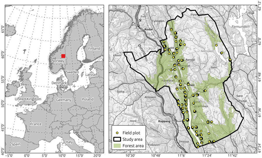
Fig. 1. Location of study area, Rendalen municipality, Innlandet county, eastern Norway, and distribution of field plots.
2.1.1 Field data
To enable the establishment of ground reference data for model calibration, field measurements were carried out on 241 field plots during summer 2015. The plots were positioned using Topcon Hiper V global navigation satellite systems (GNSS) receivers and the RTKLIB open-source software version 2.4.2 developed by Takasu (2013) was used for post-processing the recorded field plot center coordinates.
For each plot, species and diameters at breast height (dbh) were measured for trees with a dbh larger than 5 cm. Tree heights were measured using a Vertex hypsometer on sample trees selected with a probability proportional to stem basal area. On average, there were 8.5 sample trees per plot. From the field registrations, four forest attributes were calculated for each plot: plot basal area (G), plot volume (V), basal area-weighted mean height (HL), and dominant height (HO) (units can be found in Table 1). These attributes were used as response variables in the analyses. G was calculated from single tree basal areas calculated from dbh, that were summed and scaled to m2 per hectare. Plot-wise V was predicted using a ratio estimator calibrated with the height sample tree measurements, as described in (Ørka et al. 2018). In detail, the procedure was as follows:
• For all trees, a standardized tree height in meters (sh) was computed based on field measured dbh (cm) using the models published by Fitje and Vestjordet (1977).
• For all trees, a standardized volume in liters (sv) was calculated using sh and field measured dbh as input to the species-wise volume models of Vestjordet (1967), Brantseg (1967), and Braastad (1966) for spruce, pine, and deciduous species, respectively.
• For all sample trees, field reference volumes in liters (fv) were calculated using the field-measured tree height and dbh as input.
• For all sample trees, the ratio (k) between fv and sv was calculated.
• For each plot, species-wise ratio estimators (K) were calculated as the mean of k.
• For all trees, volume predictions (v) were obtained by multiplying sv to the appropriate K.
• For each plot, total volume (V) was obtained as the sum of v and scaled to m3 per hectare.
Since the sample trees were selected with a probability proportional to stem basal area, HL for each plot was obtained as the mean height of the sample trees. However, the sample of trees was not designed for a direct calculation of HO. Thus, single tree heights were predicted utilizing the above-mentioned volume models, with dbh and v as input and solving for tree height. Then, HO was estimated as the mean predicted height of the two largest trees according to dbh. Mean values and corresponding standard deviations are displayed in Table 1.
| Table 1. Number of plots (n), mean values ( | ||||||
| Acquisition year | Stratum | n | m3 ha–1 | m2 ha–1 | m | m |
| 2015 | 1 | 72 | 187 (114) | 24.4 (11.1) | 15.5 (3.4) | 19.0 (3.6) |
| 2015 | 2 | 80 | 135 (95) | 17.4 (10.2) | 15.2 (3.4) | 17.4 (3.7) |
| 2015 | 3 | 78 | 119 (87) | 17.6 (10.1) | 12.4 (2.9) | 15.3 (3.4) |
| 2015 | All | 230 | 146 (103) | 19.7 (10.4) | 14.3 (3.2) | 17.2 (3.6) |
| 2018 | 1 | 15 | 206 (118) | 25.8 (11.9) | 16.7 (2.7) | 19.5 (3.1) |
| 2018 | 2 | 12 | 204 (105) | 24.4 (9.9) | 17.2 (3.1) | 19.7 (3.0) |
| 2018 | 3 | 18 | 150 (80) | 21.3 (9.3) | 13.4 (2.3) | 16.7 (2.5) |
| 2018 | All | 45 | 183 (102) | 23.6 (10.3) | 15.5 (3.2) | 18.4 (3.1) |
2.1.2 Stratification
The field plots were stratified according to dominant tree species and development stage, which is common in operational forest management inventories to enhance the accuracy and precision of the model predictions. In the current study, we used three strata where strata 1 and 2 comprised mature spruce forests and mature pine forests, respectively, and stratum 3 was composed of young forests irrespective of species. Mature and young forests were defined according to age and productivity, where the latter was quantified using anamorphic site index (SI) models for Norway, based on tree height at an index age of 40 years determined at breast height (Tveite 1977; Sharma et al. 2011). The forest was classified as mature if total age exceeded 45 years for the most productive sites (SI = 20 m) and 85 years for the poorest sites (SI = 6 m), with a linearly increasing threshold age for the site indices in between. If the age threshold was not met, the forest was classified as young. However, regeneration forests were excluded, and the total age thresholds used to separate young- and regeneration forests were between 20 years (SI = 20 m) and 55 years (SI = 6 m).
2.2 Remotely sensed data
2.2.1 Airborne laser scanning data
The ALS data available for the area were collected as part of eight different acquisition projects run by the Norwegian mapping authority when establishing the national detailed elevation model. All data were collected using Riegl ALS instruments. The data were collected in 2016, 2017, and 2018 under leaf-on conditions. The mean point density was 3.6 points m–2 and varied from 2 to 5 points m–2.
In total, eight field plots were covered by two acquisitions, and these were handled as separate independent observations, i.e., 16 independent observations. The mean number of field plots covered by the different acquisitions was 31 and varied between 3 and 90. The lidR package (Roussel et al. 2020) was used with the TIN (Triangulated Irregular Network) option to create a triangular terrain model from the ground points and to compute a normalized point cloud (heights above the TIN).
2.2.2 Aerial images
In 2015, aerial images were acquired for the whole study area between June 11 and September 29. The average flying altitude was 5087 m, and a Vexcel UtraCam XP camera was used. The side and forward overlaps between images were 20% and 80%, respectively. The ground sampling distance of the images was 25 cm.
The second aerial image acquisition was carried out on May 24, 2018, using av Vexcel UltraCam Eagle M3 camera. The average flying altitude was 2885 m. The side and forward overlaps between images were 20% and 60%, respectively. The ground sampling distance was 10 cm. The images acquired in 2018 covered 70 of the field plots.
The Vexcel sensors acquired both panchromatic and four multispectral bands (red, green, blue, and infrared). The sensor location and orientation during image acquisitions were logged using GNSS and an inertial navigation system (INS).
2.3 Image processing
The images were processed five times, using four different image matching software packages. Match-T was used twice (labeled MatchT1 and MatchT2), by two different institutions. As a result, five sets of point clouds were generated by image matching. The different matching routines are defined as follows:
• Agisoft
• MatchT1
• MatchT2
• Pix4DMapper (henceforth: Pix4D)
• SURE
Using the software Match-AT, we computed the exterior orientation (EO) of the images once, and then used this result for all subsequent matching routines. An initial EO was first determined using a combination of the INS and GNSS that was onboard the sensor platform at the time of data acquisition. The initial EO was further improved using ground control points. Finally, an unbiased estimate of the quality of the final EO was computed using checkpoints. As the checkpoints were not involved in the computation of the EO, they provide the most unbiased method of estimating the EO accuracy.
Ultimately, 24 ground control points were used for the 2015 dataset, and 11 for the 2018 dataset. One checkpoint was used for the 2015 dataset, and two for the 2018 dataset. It is worth noting that additional ground control points and checkpoints were in fact used to optimize the EO. However, only those residing within our study area were considered here, as they were the most relevant.
The interior orientation (IO) of the images, also known as the sensor calibration parameters, was computed before the data acquisition through a lab calibration routine executed by the sensor’s manufacturer. The calibration results were used as the initial IO in all matching routines. Except for the Agisoft routine, no further optimization of the initial IO was done, resulting in identical IO for all but the Agisoft routine. However, it is worth noting that reformatting and transforming the IO files resulting from Match-AT was required before using them in other software. This is due to the differences in input formats and sensor coordinate systems from one software to another. Unlike other routines, the Agisoft routine did permit additional optimization of the IO. This led to minor variations in the IO parameters used by Agisoft compared to other routines, but these variations were deemed not important.
Carrying out image matching across different routines presented a challenge due to the difficulty in maintaining identical processing settings. The reason being that each software utilizes unique terminology and parameters, which affect properties such as the number of image pixels matched, image scaling, and any smoothing applied to the results. Nonetheless, we strived to ensure that each routine’s image matching process was performed in a way that was as comparable as possible to the others. The output for each processing routine was one set of point cloud files for each routine.
For each set of point cloud files, the lidR package (Roussel et al. 2020) with the TIN option was used for calculating the heights above the ground calculated from ALS-classified ground echoes. These normalized point clouds from the five routines and the normalized ALS point cloud form the point cloud types used for the analyses.
2.4 Selection of data for the analyses
The analyses were carried out on two separate datasets defined by the acquisition years of the aerial imagery (2015 and 2018). The field data comprised 241 field plots inventoried in 2015. However, the 2015 dataset was reduced to 230 plots. For the 11 excluded plots, at least one the image matching routines failed to produce a point cloud; no obvious reason for the failure was identified. The 2018 images covered 70 of the field plots. Five of these plots were discarded from the analysis because they were harvested prior to the date when the images in 2018 were acquired. For the remaining 65 plots, there were only 45 plots, from which point clouds were obtained with all the matching routines. The analyses were conducted using only the plots for which all point cloud types were represented.
2.5 Metrics
For each plot, canopy height metrics were calculated for each point cloud, both image matching and ALS. The set of metrics comprised percentiles at 10% intervals (H10, H20, ..., H90) calculated from points exceeding a threshold of 2 m above ground. In addition, we computed the mean height (Hmean), standard deviation (Hsd), coefficient of variation (Hcv), kurtosis (Hkurt), and skewness (Hskewness) using the same threshold. Furthermore, canopy density metrics were calculated. First, the 0, 1, …, 9th deciles of the height range between the 2 m threshold and the 95% height percentile were calculated. Then, the number of echoes above each decile-height was divided by the total number of echoes from the plot (including echoes below the threshold), resulting in ten canopy density metrics (D0, D1, ..., D9).
2.6 Analyses
For each response variable (G, V, HL, and HO), models were constructed based on metrics representing the properties of each point cloud. In total, 144 models were constructed (four response variables, three strata, six point cloud types, and two acquisition years). Both the response and explanatory variables were transformed using the natural logarithm (ln), and linear models were fitted using ordinary least squares. Variable selection was conducted using the regsubsets function from the leaps package in R (Lumley and Miller 2024), with the model that exhibited the smallest Bayesian information criterion (BIC) being retained. However, to control for multicollinearity, additional constraints were implemented: the maximum number of explanatory variables was limited to three, and the variance inflation factor (Montgomery et al. 2013) was not allowed to exceed the value of 2. Because the response variables were ln-transformed, the model intercept was adjusted for logarithmic bias by adding half of the model variance to the intercept (Goldberger 1968). Subsequently, the models were applied for prediction to their respective strata, and the differences (D) between the back-transformed predicted values and field reference values were calculated.
For each model, the relative root mean square error (RMSE%) was calculated as:
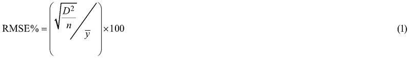
where n is the number of field reference plots used to construct the model and ![]() is the mean field reference value.
is the mean field reference value.
We analyzed the distributions of RMSE% related to each type of point cloud for the entire range of field plots, but also for subsets per stratum and per variable. However, we kept data from the different acquisition years separate because the 2018 dataset was a subdivision of the 2015 dataset. Two types of analyses were conducted. The distributions were first assessed visually, by means of boxplots, to evaluate the magnitude of RMSE% and the differences between the models. This assessment was made for the entire range of field plots and per response variable.
Secondly, to determine if there were statistically significant differences in model performance, Tukey’s honestly significant difference tests (HSD tests) (Tukey 1949) were applied to the absolute, relative differences (|rD|) between predicted and field reference values, calculated as follows:

This analysis focuses on the magnitude of D and tests whether a specific model is associated with larger or smaller random errors, compared to the other models tested. This analysis was carried out both for the entire dataset, and separately for each individual stratum and variable.
3 Results
3.1 Modelling
All models described in paragraph 2.6 are presented in Supplementary file S1, which includes their selected explanatory variables, R2 values, p-values from t-tests on the residuals, percentage standard deviations of the residuals, and the corresponding percentage root mean square values. Summarized results (Table 2) show that the selected metrics for V and G cover the complete range. However, the upper-range percentiles (H60–Hmax) and lower-range density metrics (D0–D4) were chosen more frequently irrespective of point cloud type.
| Table 2. Occurance of different types of metrics in the models, percentages of models having one and two explanatory variables, and the range of accuray expressed as relative RMSE. The results are distributed between point cloud types and response variable categories (Vars) grouping the density dependent G and V together as well as the height variables (HL and HO). | ||||||||||
| Point cloud type | Vars | Occurance of metrics (%) *1 | Number of metrics (%) *2 | Range in accuracy (%) | ||||||
| Density metrics | Heigh percentiles | Mom. Stat. *7 | ||||||||
| Lower range *3 | Upper range *4 | Lower range *5 | Upper range *6 | One | Two | Min RMSE | Max RMSE | |||
| Image | G, V | 15 | 21 | 13 | 43 | 8 | 47 | 53 | 21.3 | 40.2 |
| ALS | G, V | 38 | 13 | 8 | 21 | 21 | 0 | 100 | 19.3 | 25.7 |
| Image | HL, HO | 11 | 5 | 8 | 66 | 11 | 73 | 27 | 9.2 | 16.3 |
| ALS | HL, HO | 25 | 0 | 0 | 75 | 0 | 67 | 33 | 8.7 | 11.5 |
| *1: The numbers are percentages of the total number of metrics selected for the models represented on each line in the table. *2: The numbers are percentages of the total number of models represented on each line in the table. *3: D0–D4. *4: D5–D9. *5: H10–H50. *6: H60–Hmax. *7: Moment statistics (Hmean, Hsd, Hcv, Hkurt, Hskewness) | ||||||||||
For HO and HL, the models predominantly feature upper-range percentiles (H60–Hmax), although additional metrics across a broader spectrum were sometimes selected.
In terms of the number of explanatory variables, the models were evenly split between those incorporating one explanatory variable and those comprising two. There were more ALS models including two metrics compared to those based om image matching data. Thus, the image matching models had fewer explanatory variables than the ALS models. Furthermore, models for the height responses had fewer explanatory variables than those for V and G.
The model fit, as indicated by R2, ranged from 0.59 to 0.97 for V and G, while the height responses exhibited R2 values between 0.47 and 0.95 (Suppl. file S1). The average R2-values for both these two groups of responses were both slightly larger for ALS models compared to those based on image matching data. For the V and G group, the mean R2 value was 0.80 for ALS models and 0.72 for image matching models. Corresponding values for the height responses were 0.86 and 0.74, respectively. The RMSE%-values were generally smaller for ALS compared to image matching and smaller for height variables compared to G and V (Table 2).
3.2 Visual assessment of RMSE% distributions
Models utilizing ALS point clouds displayed both smaller median RMSE% and less variation compared to those based on image matching point clouds (Fig. 2). It can also be noted that the median RMSE% values resulting from the 2018 analysis were on a slightly lower level compared to those based on the 2015 dataset.
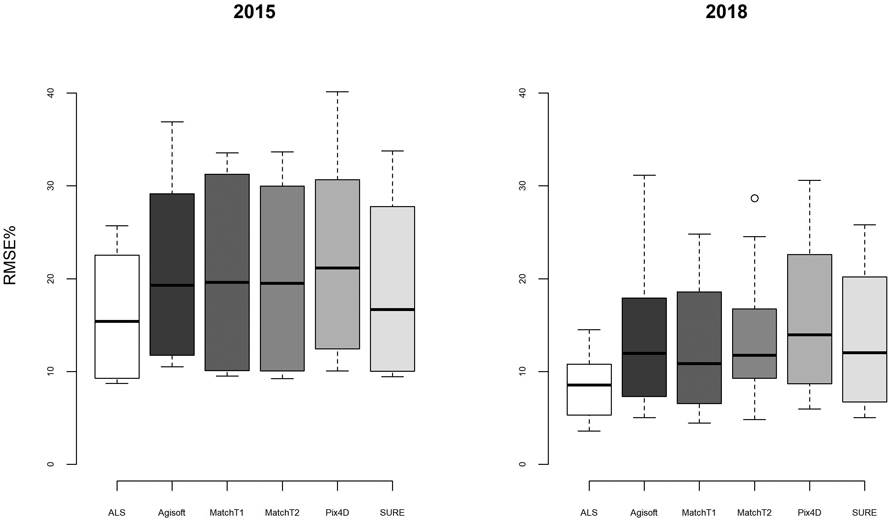
Fig. 2. Distributions of RMSE% associated with models constructed using explanatory variables calculated from different point cloud types on the 2015 (left panel) and 2018 datasets (right panel).
The results categorized by response variables (Fig. 3) showed that there was notably greater variation among point cloud types than seen in the overall results. For the variables with per hectare units, i.e., G and V, ALS-based models displayed substantially smaller values of median and range of RMSE% compared to the models based on image matching point clouds. Among these visualized results based on the image matching point clouds, there are no clear indications that the different processing routines yield different results in terms of precision. Their performances seem to vary among response variables.
For the height responses, unlike the G and V results, the median values associated with ALS were in many cases closer to those related to image matching. The median values for all point cloud types were similar for HO but exhibited larger variation for HL.
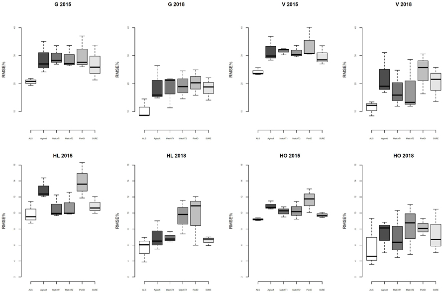
Fig. 3. Distributions of RMSE% specific to each response variable associated with models constructed using explanatory variables calculated from different point cloud types (labels on x-axes) on the 2015 and 2018 datasets. View larger in new window/tab.
3.3 HSD tests
The HSD tests conducted on the absolute, relative differences (|rD|) revealed statistically significant differences in model performance based on ALS compared to all other types of point clouds (Fig. 4). The bars (Fig. 4) represent the proportion of HSD tests that identified significant differences in |rD| among all combinations of point cloud types. For each combination of point cloud types, the figure summarizes 16 HSD tests carried out separately for three strata and four variables for each of the two acquisition years, plus one overall test for each year independent of stratum and variable. Altogether there were 240 HSD tests (Suppl. file S2). Tests performed at both the stratum and variable levels indicated that |rD| values obtained from application of ALS models were for the most part significantly different (smaller) than those from other point cloud types. In contrast, among the models based on image matching point clouds, only a few significant differences were observed (Pix4D vs MatchT1 and SURE).
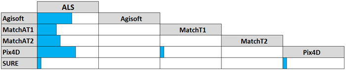
Fig. 4. Summary of Tukey HSD tests of |rD| resulting from comparing predictions from different point cloud types on different subsets of data. Bars indicate the proportion of 16 tests that identified statistically significant differences in |rD| among all combinations of point cloud types separately for the two acquisition years.
4 Discussion
The primary findings of the current study indicate that models of forest attributes constructed using ALS point cloud metrics, exhibit substantially smaller RMSE compared to those relying on metrics derived from image matching point clouds. Our results suggest that these differences are more pronounced for V and G than for the height variables HL and HO. The differences between the models based on metrics from image matching point cloud were, for the most part, negligible.
It was expected that different explanatory variables would be chosen for the models based on different point cloud types, as these datasets possess distinct inherent properties. Nevertheless, from a standpoint of biophysical consistency, we had certain expectations regarding which metrics that should be selected. For example, based on field-measured variables, V can be predicted as a function of mean tree height and stand density, typically represented by basal area. Thus, effective explanatory variables obtained from remotely sensed data often include a height percentile from the upper part of the canopy, along with a density metric. However, the combinations may vary depending on the characteristics of the field reference data and the remotely sensed datasets.
The observation that image matching models included a broader range of metrics than those based on ALS metrics, can be attributed to the narrower height range of image matching point clouds. These point clouds often fail to capture points deep within the canopy, as such points are unlikely to be represented in a single image, let alone across multiple images. Consequently, image matching point clouds tend to smooth gaps in the canopy (White et al. 2018), primarily representing the canopy surface, thereby resulting in a narrower range of calculated metrics. In contrast, ALS offers a more complete depiction of the vertical forest structure, yielding metrics that are less uniformly selected across the height range. The predominance of canopy surface representation in image matching point clouds poses considerable challenges, particularly in light of the increasing demand for uneven-aged forests and continuous cover forestry, in line with the revised PEFC standard (PEFC 2022). Decision making under such management regimes, typically requires information from deeper levels of the canopy (Mehtätalo et al. 2024).
The current study also highlighted that the coverage of image matching point data across the area of interest may be incomplete and influenced by the specific software used for matching. In the context of forest inventory, which relies on wall-to-wall remotely sensed data, this is a challenge. In the current study, the plots for which image matching point clouds were missing were not the same among the different software packages. Furthermore, our data did not allow analyses to uncover the underlying reasons for these discrepancies. Future research should investigate the various software algorithms, the quality and resolution of the input imagery, and environmental conditions that may impact data acquisition.
An analysis of the RMSE% resulting from the various models indicates that models based on ALS metrics generally demonstrated greater precision compared to their image matching counterparts (Figs. 2 and 3). This pattern remained consistent across all data subsets. Other studies have found similar trends, although some reported only minor differences between ALS and image matching metrics. For instance, Nurminen et al. (2013) reported RMSE% values of 22.6 and 6.8 for volume and mean height using image matching, respectively, compared to 20.7 and 6.6 for ALS in the current study. Similarly, Gobakken et al. (2015) observed minimal differences between data sources. More substantial contrasts between these two methods were documented by Järnstedt et al. (2012), Straub et al. (2013), and Vastaranta et al. (2013). In the current study, considering the full range of plots (2015 data), we found at least a five-percentage-point difference in RMSE% values between ALS and any of the image matching results for volume. This aligns with findings from the aforementioned studies. Although Järnstedt et al. (2012) found a relatively large RMSE% difference for mean height as well, the current study found a difference of less than one-percentage-point between ALS and the image matching point cloud type that yielded the smallest RMSE% value (MatchT1). As Vastaranta et al. (2013) point out, forest attributes that are strongly dependent on forest density (V and G) may be more prone to be poorly modelled using image matching data. This is most likely the explanation for the greater difference between ALS and image matching for these variables in the current study.
The HSD tests revealed statistically significant differences between the |rD| values related to the ALS models and most of the corresponding models based on image matching metrics. There were, however, only a few statistically significant |rD| among the models based on image matching point clouds. These few significant differences were obtained on stratum level. No significant differences were observed at the level of the different response variables (Suppl. file S2), even though there were striking visual differences in the RMSE% distributions for HL (Fig. 3). Thus, there was no concrete evidence that that the different image matching routines yielded different results.
5 Conclusion
The findings of the current study revealed advantages in using ALS point clouds over those generated using image matching. Furthermore, the results indicated that there were no differences in the qualities among those models based on metrics calculated from image matching point clouds. The results indicated that ALS point clouds are better suited to represent complex forest structures. As forest management increasingly necessitates detailed information from various canopy layers, it is crucial to understand the limitations of image matching techniques. Future research should focus on enhancing the knowledge on the properties of different types of point cloud data and developing optimal modeling strategies that align with diverse forestry management goals.
Declaration of openness of research materials, data, and code
The field data used in the current study are not openly available. The images used for creating the image matching point clouds are available from https://www.norgeibilder.no/. The airborne laser scanner data are available from https://hoydedata.no. Codes used in the study can be made available by reasonable request by e-mail to the first author.
Authors’ contributions
Ole Martin Bollandsås: data analyses, interpretation of results, visualization, writing of original draft, review and editing. Terje Gobakken: conceptualization of original idea, funding acquisition, interpretation of results, project management, review and editing, writing. Erik Næsset: funding acquisition, interpretation of results, review and editing. Bjørn-Eirik Roald: data curation, processing of remotely sensed data, review and editing, writing. Hans Ole Ørka: coding for data analyses, conceptualization of original idea, data curation, project management, review and editing, writing.
Declaration of the use of generative artificial intelligence and AI-assisted technologies in the writing process
Chat-GPT was utilized to rephrase individual sentences. The final text has been carefully reviewed to confirm that the meaning aligns with the intended message.
Acknowledgements
The authors want to thank Glommen-Mjøsen Skog SA, for making the field data available for the study.
Funding
This work is part of the Center for Research-based Innovation SmartForest: Bringing Industry 4.0 to the Norwegian forest sector (NFR SFI project no. 309671, smartforest.no).
References
Alidoost F, Arefi H (2017) Comparison of UAS-based photogrammetry software for 3D point cloud generation: a survey over a historical site. ISPRS Ann Photogramm Remote Sens Spatial Inf Sci IV-4/W4: 55–61. https://doi.org/10.5194/isprs-annals-IV-4-W4-55-2017.
Braastad H (1966) Volume tables for birch. Medd Nor Skogforsøksvesen 21: 23–78.
Brantseg A (1967) Volume functions and tables for Scots pine: South Norway. Medd Nor Skogforsøksvesen 22: 689–739.
Fitje A, Vestjordet E (1977) Stand height curves and new tariff tables for Norway spruce. Medd Norsk Inst Skogforsk 34: 23–68.
Gobakken T, Bollandsås OM, Næsset E (2015) Comparing biophysical forest characteristics estimated from photogrammetric matching of aerial images and airborne laser scanning data. Scand J For Res 30: 73–86. https://doi.org/10.1080/02827581.2014.961954.
Goldberger AS (1968) The interpretation and estimation of Cobb-Douglas functions. Econometrica 36: 464–472. https://doi.org/10.2307/1909517.
Harshit KJ, Zlatanova S (2023) Advancements in open-source photogrammetry with a point cloud standpoint. Appl Geomat 15: 781–794. https://doi.org/10.1007/s12518-023-00529-4.
Järnstedt J, Pekkarinen A, Tuominen S, Ginzler C, Holopainen M, Viitala R (2012) Forest variable estimation using a high-resolution digital surface model. ISPRS J Photogramm Remote Sens 74: 78–84. https://doi.org/10.1016/j.isprsjprs.2012.08.006.
Korpela I (2004) Individual tree measurements by means of digital aerial photogrammetry. Silva Fenn Monogr 3. https://doi.org/10.14214/sf.sfm3.
Loetsch F, Haller KE, Brünig EF (1964) Forest inventory. Vol. 1: Statistics of forest inventory and information from aerial photographs. BVL Verlagsgesellschaft, München, Germany.
Lumley T, Miller A (2024) leaps: regression subset selection. R Package, version 3.2. https://CRAN.R-project.org/package=leaps.
Maltamo M, Næsset E, Vauhkonen J (eds) (2014) Forestry applications of airborne laser scanning. Concepts and case studies. Springer Dordrecht, Managing Forest Ecosystems 27. https://doi.org/10.1007/978-94-017-8663-8.
Mehtätalo L, Kangas A, Eggers J, Eid T, Eyvindson K, Lundström J, Siipilehto J, Öhman K (2024) Forest planning and continuous cover forestry. In: Rautio P, Routa J, Huuskonen S, Holmström E, Cedergren J, Kuehne C (eds) Continuous cover forestry in boreal nordic countries. Springer, Cham, Managing Forest Ecosystems 45: 93–107. https://doi.org/10.1007/978-3-031-70484-0_5.
Montgomery D, Peck E, Vining G (2013) Introduction to linear regression analysis. John Wiley & Sons, Inc., Hoboken, New Jersey. ISBN 978-0-470-54281-1.
Niederheiser R, Mokroš M, Lange J, Petschko H, Prasicek G, Elberink SO (2016) Deriving 3D point clouds from terrestirial photographs – comparison of different sensors and software. Int Arch Photogramm Remote Sens Spatial Inf Sci XLI-B5: 685–692. https://doi.org/10.5194/isprs-archives-XLI-B5-685-2016.
Nurminen K, Karjalainen M, Yu X, Hyyppä J, Honkavaara E (2013) Performance of dense digital surface models based on image matching in the estimation of plot-level forest variables. ISPRS J Photogramm Remote Sens 83: 104–115. https://doi.org/10.1016/j.isprsjprs.2013.06.005.
Næsset E (2002a) Determination of mean tree height of forest stands by digital photogrammetry. Scand J For Res 17: 446–459. https://doi.org/10.1080/028275802320435469.
Næsset E (2002b) Predicting forest stand characteristics with airborne scanning laser using a practical two-stage procedure and field data. Remote Sens Environ 80: 88–99. https://doi.org/10.1016/S0034-4257(01)00290-5.
Ørka HO, Bollandsås OM, Hansen EH, Næsset E, Gobakken T (2018) Effects of terrain slope and aspect on the error of ALS-based predictions of forest attributes. Forestry 91: 225–237. https://doi.org/10.1093/forestry/cpx058.
PEFC (2022) Norwegian PEFC forest standard. https://pefc.no/vare-standarder/norsk-pefc-skog-standard.
Roussel JR, Auty D, Coops NC, Tompalski P, Goodbody TRH, Meador AS, Bourdon JF, de Boissieu F, Achim A (2020) lidR: an R package for analysis of Airborne Laser Scanning (ALS) data. Remote Sens Environ 251, article id 112061. https://doi.org/10.1016/j.rse.2020.112061.
Sharma RP, Brunner A, Eid T, Øyen BH (2011) Modelling dominant height growth from national forest inventory individual tree data with short time series and large age errors. For Ecol Manag 262: 2162–2175. https://doi.org/10.1016/j.foreco.2011.07.037.
Spurr SH (1952) Aerial photographs in forest management. Photogrammetria 9: 33–41. https://doi.org/10.1016/S0031-8663(52)80004-3.
St‐Onge B, Vega C, Fournier RA, Hu Y (2008) Mapping canopy height using a combination of digital stereo‐photogrammetry and lidar. Int J Remote Sens 29: 3343–3364. https://doi.org/10.1080/01431160701469040.
Standish M (1945) The use of aerial photographs in forestry. J For 43: 252–257. https://doi.org/10.1093/jof/43.4.252.
Straub C, Stepper C, Seitz R, Waser LT (2013) Potential of UltraCamX stereo images for estimating timber volume and basal area at the plot level in mixed European forests. Can J For Res 43: 731–741. https://doi.org/10.1139/cjfr-2013-0125.
Takasu T (2013) RTKLIB, version 2.4.2 manual. https://www.rtklib.com/prog/manual_2.4.2.pdf.
Tukey JW (1949) Comparing individual means in the analysis of variance. Biometrics 5: 99–114. https://doi.org/10.2307/3001913.
Tveite B (1977) Bonitetskurver for gran. Medd Norsk Inst Skogforsk 33: 1–84.
Vastaranta M, Wulder MA, White JC, Pekkarinen A, Tuominen S, Ginzler C, Kankare V, Holopainen M, Hyyppä J, Hyyppä H (2013) Airborne laser scanning and digital stereo imagery measures of forest structure: comparative results and implications to forest mapping and inventory update. Can J Remote Sens 39: 382–395. https://doi.org/10.5589/m13-046.
Vestjordet E (1967) Functions and tables for volume of standing trees. Norway spruce. Medd Nor Skogforsøksvesen 22: 539–574.
White JC, Coops NC, Wulder MA, Vastaranta M, Hilker T, Tompalski P (2016) Remote sensing technologies for enhancing forest inventories: a review. Can J Remote Sens 42: 619–641. https://doi.org/10.1080/07038992.2016.1207484.
White JC, Tompalski P, Coops NC, Wulder MA (2018) Comparison of airborne laser scanning and digital stereo imagery for characterizing forest canopy gaps in coastal temperate rainforests. Remote Sens Environ 208: 1–14. https://doi.org/10.1016/j.rse.2018.02.002.
Total of 33 references.
